- Research Article
- Open access
- Published:
Stability of Linear Dynamic Systems on Time Scales
Advances in Difference Equations volume 2008, Article number: 670203 (2008)
Abstract
We examine the various types of stability for the solutions of linear dynamic systems on time scales and give two examples.
1. Introduction
Continuous and discrete dynamical systems have a number of significant differences mainly due to the topological fact that in one case the time scale  , real numbers, and the corresponding trajectories are connected while in other case
  , integers, they are not. The correct way of dealing with this duality is to provide separate proofs. All investigations on the two time scales show that much of the analysis is analogous but, at the same time, usually additional assumptions are needed in the discrete case in order to overcome the topological deficiency of lacking connectedness. Thus, we need to establish a theory that allows us to handle systematically both time scales simultaneously. To create the desired theory requires to setup a certain structure of
  which is to play the role of the time scale generalizing
  and
and  . Furthermore, an operation on the space of functions from
  to the state space has to be defined generalizing the differential and difference operations. This work was initiated by Hilger [1] in the name of "calculus on measure chains or time scales."
In this paper, we examine the various types of stability-stability, uniform stability, asymptotic stability, strong stability, restrictive stability, and so forth, for the solutions of linear dynamic systems on time scales and give two examples.
2. Preliminaries on Dynamic Systems
We mention without proof several foundational definitions and results in the calculus on time scales from an excellent introductory text by Bohner and Peterson [2]. A time scale is a nonempty closed subset of
  , and the forward jump operator
 is defined by

(supplemented by  ), while the graininess
 is given by

If has a left-scattered maximum  , then
  and otherwise
  . A function
  is called differentiable at
  , with (delta) derivative
 if given
  there exists a neighborhood
  of
of  such that, for all
  ,
,

where  .
.
Some basic properties of delta derivatives are given in the following [3–5]:
-
(i)
If
 is differentiable at
  , then
  (2.4)
(2.4) -
(ii)
If both
 and
and  are differentiable at , then the product
  is also differentiable at with
  (2.5)
(2.5)
 is differentiable at
  , then
 and
and  are differentiable at
  is also differentiable at
A function  is said to be rd-continuous (denoted by
  if
if
-
(i)
 is continuous at every right-dense point
  ,
, -
(i)
 exists and is finite at every left-dense point .
 is continuous at every right-dense point
  ,
, exists and is finite at every left-dense point
 A function  is called an antiderivative of
  on if it is differentiable on and satisfies
  for
for  . In this case, we define

where  .
.
The norm of an  matrix
  is defined to be

where  is the
  th column of
  .
.
Let  be the set of all
  matrices over
  . The class of all rd-continuous and regressive functions
  is denoted by

Here, a matrix-valued function  is called regressive provided:

where  is the identity matrix.
Definition 2.1.
Let  . The unique matrix-valued solution of the IVP

where  , is called the matrix exponential function and it is denoted by
  .
.
3. Stability of Linear Dynamic Systems
We consider the dynamic system

where  with
with  and
and  is the delta derivative of
  with respect to
  . We assume that the solutions of (3.1) exist and are unique for
  , and is unbounded above.
We give the definitions about the various types of stability for the solutions of (3.1).
Definition 3.1.
The solution  of (3.1) is said to be stable if, for each
  , there exists a
  such that, for any solution
  of (3.1), the inequality
  implies
  for all
  .
.
Definition 3.2.
The solution  of (3.1) is said to be uniformly stable if, for each
  , there exists a
  such that, for any solution
  of (3.1), the inequalities
  and
and  imply
imply  for all
  .
.
Definition 3.3.
The solution  of (3.1) is said to be asymptotically stable if it is stable and there exists a
  such that
  implies
  as
as  .
.
The following notion of strong stability is due to Ascoli [6].
Definition 3.4.
The solution  of (3.1) is said to be strongly stable if, for each
  , there exists a
  such that, for any solution
  of (3.1), the inequalities
  and
and  imply
imply  for all
  .
.
For the other types of stability, that is,  -stability, we refer to [7].
We note that the stability of any solution of (3.1) is closely related to the stability of the null solution of the corresponding variational equation. Therefore, we will discuss the stability of linear dynamic system.
We consider the linear homogeneous dynamic system

where  .
.
It follows that any solution of the linear dynamic system is (uniformly, strongly, asymptotically) stable if and only if the same holds for the zero solution of (3.2). We say that (3.2) is (uniformly, strongly, asymptotically stable) stable if so is the null solution of (3.2). See [8].
Firstly, we show that the stability for solutions of (3.2) is equivalent to the boundedness.
Theorem 3.5.
Equation (3.2) is stable if and only if all solutions of (3.2) are bounded for all  .
.
Proof.
Suppose that (3.2) is stable. Since the trivial solution  is stable, given any
  , there exists a
  such that
  implies
  . Note that
  for all
  . Now, let
  be a vector of length
  in the
  th direction for
  . Then,
  , where
  is the
  th column of
  . Thus, we have

Consequently, for any solution  of (3.2),

It follows that all solutions of (3.2) are bounded.
For the converse, we note that all solutions of (3.2) are bounded if and only if there exists a positive constant  such that

It follows from  that (3.2) is stable. This completes the proof.
In [9, Theorem 2.1], DaCunha obtained the following characterization of uniform stability by means of the operator norm. It is not difficult to prove this result by using the maximum norm.
Theorem 3.6.
Equation (3.2) is uniformly stable if and only if there exists a positive constant  such that

for all  with
with  .
.
The following is the characterization of strong stability for linear dynamic system (3.2). Note that its continuous version was presented in [10].
Theorem 3.7.
Equation (3.2) is strongly stable if and only if there exists a positive constant  such that

where  is a matrix exponential function of (3.2).
Proof.
Suppose that (3.7) holds. For any given  , we can choose
  such that for any
  ,
,  . Then, we have

Hence, (3.2) is strongly stable.
Conversely, if (3.2) is strongly stable, then we have

whenever  and
and  holds. Since
  is arbitrary, we have

where  . It is clear that
  , and hence
  , is independent of
  and
and  as well as of
  . Putting
  and
and  , we obtain the result.
Example 3.8 (see [8]). (i) The system  is strongly stable, but it is not asymptotically stable.
(ii) The system  with
with  is asymptotically stable, but it is not strongly stable.
Restrictive stability in [10] is related to strong stability, and we obtain their equivalence for (3.2) as a consequence of Theorem 3.7.
Definition 3.9.
System (3.2) is said to be restrictively stable if it is stable and its adjoint system

where  denotes the conjugate transpose of
  , is stable.
Remark 3.10.
We note that (3.2) is strongly stable if and only if it is restrictively stable.
Definition 3.11.
System (3.2) is said to be reducible (or reducible to zero), if there exists  which is bounded together with its inverse
  on
on  such that
  is a constant (or zero) matrix on . Here,
  , and the set of all functions
  that are differentiable and whose derivative is rd-continuous is denoted by

Theorem 3.12.
System (3.2) is restrictively stable if and only if it is reducible to zero.
Proof.
Let  be a matrix exponential function of (3.2). Suppose that (3.2) is restrictively stable. Then, there exists a positive constant
  such that

by means of Theorem 3.7. Consider the transformation  . Then, it follows that

Hence, we obtain

since  . This implies that (3.2) is reducible to zero.
For the converse, suppose that there exists  such that

Then, we have  . Thus,
  is a matrix exponential function of (3.2). Since
  and
and  are bounded for all
  , the proof is complete.
Theorem 3.13.
If (3.2) is stable and reducible on a time scale with the constant graininess, then it is uniformly stable.
Proof.
Since (3.2) is reducible, we have

where  by the transformation
  . Let
. Let  be a matrix exponential function of (3.2). The stability of (3.2) implies the boundednesss of
  . Let
. Let  , where
  is a matrix exponential function of (3.17). Then, we have

and hence the boundedness of  implies the boundedness of
  since
since  is bounded. Thus, (3.17) is stable and, in fact, is uniformly stable. Hence, it is clear that

for some positive constant  and all
  . Therefore,

for some positive constant  and all
  . Consequently, (3.2) is uniformly stable.
The continuous versions of Theorems 3.12 and 3.13 are presented in (3.9.v) and (3.9.vi) in [10], respectively.
Remark 3.14.
It does not hold in general that every stable linear homogeneous system with constant coefficient matrix on a time scale is uniformly stable.
Corollary 3.15.
If (3.11) is stable and  with the eigenvalues
  (
( ) of
) of  , then it is restrictively stable.
Proof.
It follows from the stability of (3.2) that  is bounded for all
  . Furthermore, by Liouville's formula [11], we have

where  is a positive constant. Thus, from

it is clear that  is bounded for all
  . The proof is complete.
Remark 3.16.
Pötzsche et al. [12] proved a necessary and sufficient condition for the exponential stability of time-variant linear systems on time scales in terms of the eigenvalues of the system matrix. They used a representation formula for the transition matrix of Jordan reducible systems in the regressive case.
Remark 3.17.
In summary, the following assertions are all equivalent [13, Theorem 4.2].
-
(i)
System (3.2) is strongly stable.
-
(ii)
There exists a positive constant
 such that
  (3.23)
 -
(iii)
Adjoint system (3.11) of (3.2) is strongly stable.
-
(iv)
System (3.2) is restrictively stable.
-
(v)
System (3.2) is reducible to zero.
 such that
It is widely known that the stability characteristics of a nonautonomous linear system of differential or difference equations can be characterized completely by a corresponding autonomous linear system by the Lyapunov transformation. DaCunha and Davis in [14] gave a definition of the Lyapunov transformation as follows.
Let  . The Lyapunov transformation is an invertible matrix-valued function
  with the property that, for some positive
  ,
,

for all  .
.
Remark 3.18.
Note that the boundedness of the coefficient matrices is not preserved by the Lyapunov transformation  in the case of the time scales with right-dense point [13]. This can be seen by considering the time scale
  and the Lyapunov transformation:

It shows that the coefficient matrices  and
and  satisfy

where  and
and  .
.
Now, we consider the linear dynamic system

and its perturbed system

where  .
.
The following theorem means that the strong stability for the system (3.27) is equivalent to that of (3.2).
Lemma 3.19 (see [14, Theorem 3.8]).
Suppose that  is invertible for all
  , and
, and  is regressive. Then, the transformation matrix for the system

where

is given by

for all  .
.
The regressiveness of  in (3.30) is preserved by the Lyapunov transformation in the following lemma.
Lemma 3.20.
Suppose that
is the transformation matrix for all
 . Then
is regressive if and only if
is also regressive.
. Then
is regressive if and only if
is also regressive.
Proof.
We see that for every right-scattered point  , the following identity holds:

This completes the proof.
Theorem 3.21.
Suppose that  is a Lyapunov transformation. Then (3.2) is strongly stable if and only if (3.27) is strongly stable.
Proof.
Suppose that (3.2) is strongly stable. Then, there exists a constant  such that

By using Lemma 3.19, we have

Hence, (3.27) is strongly stable.
The converse holds similarly.
If we assume that the perturbing term  is absolutely integrable, then we obtain the uniform stability for the perturbed system (3.28) when system (3.2) is strongly stable.
Theorem 3.22.
Suppose that  is a Lyapunov transformation and there exists a
  such that for all
  :
:

If (3.2) is strongly stable, then (3.28) is uniformly stable.
Proof.
It follows from Theorem 3.21 that (3.27) is strongly stable. Then, there exists a positive constant  such that

For any  and
and  , the solution
  of (3.28) satisfies

By taking the norms of both sides of (3.37), we have

In view of Gronwall's inequality [15], we obtain

for all  . Thus

where  . Hence, (3.28) is uniformly stable.
4. Examples
In this section, we give two examples about the various types of stability for solutions of linear dynamic systems on time scales in [16].
Example 4.1.
To illustrate Theorem 3.7, we consider the linear dynamic system

where  . If
. If  for all
  , then (4.1) is strongly stable.
Remark 4.2.
We give some remarks about Example 4.1.
-
(1)
If
 , then
  of linear differential system
  is given by
 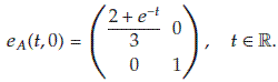 (4.2)
(4.2) -
(2)
If
 with the positive constant
  for all
  , then
  of linear difference system
  (4.3)
(4.3)is given by
 (4.4)
(4.4) -
(3)
If
 with the constant
  , then
  of
of  -difference system
 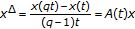 (4.5)
(4.5)is given by
 (4.6)
(4.6) -
(4)
If
 and
and 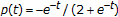 , then
  of linear dynamic system
 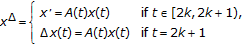 (4.7)
(4.7)is given by
 (4.8)
(4.8)
 , then
  of linear differential system
  is given by
 with the positive constant
  for all
  , then
  of linear difference system

 with the constant
  , then
  of
of  -difference system

 and
and  , then
  of linear dynamic system

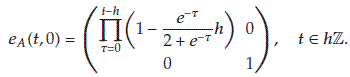
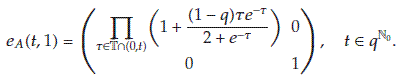
Example 4.3.
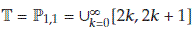
We consider the linear dynamic system

where  . If
. If  for all
  , then the matrix exponential function
  of (4.9) is given by

We see that the generalized exponential function  is given by

respectively. Thus, we obtain the following results for (4.9) and  .
.
-
(1)
If
 , then (4.9) is uniformly stable but not strongly stable.
 -
(2)
If
 , then (4.9) is strongly stable but not asymptotically stable.
 -
(3)
If
 with
with  and
and  , then (4.9) is neither asymptotically stable nor strongly stable. However,
  goes to zero as
  .
. -
(4)
If
 with
with  , then (4.9) is neither asymptotically stable nor strongly stable.
 -
(5)
If
 with
with  , then (4.9) is unbounded and
  is oscillatory.
 -
(6)
If
 , then (4.9) is bounded and
  goes to zero as
  .
.
 , then (4.9) is uniformly stable but not strongly stable.
 , then (4.9) is strongly stable but not asymptotically stable.
 with
with  and
and  , then (4.9) is neither asymptotically stable nor strongly stable. However,
  goes to zero as
  .
. with
with  , then (4.9) is neither asymptotically stable nor strongly stable.
 with
with  , then (4.9) is unbounded and
  is oscillatory.
 , then (4.9) is bounded and
  goes to zero as
  .
.References
Hilger S: Analysis on measure chains—a unified approach to continuous and discrete calculus. Results in Mathematics 1990, 18(1-2):18-56.
Bohner M, Peterson A: Dynamic Equations on Time Scales. An Introduction with Applications. Birkhäuser, Boston, Mass, USA; 2001:x+358.
Agarwal R, Bohner M, O'Regan D, Peterson A: Dynamic equations on time scales: a survey. Journal of Computational and Applied Mathematics 2002, 141(1-2):1-26. 10.1016/S0377-0427(01)00432-0
Bohner M, Hering R: Perturbations of dynamic equations. Journal of Difference Equations and Applications 2002, 8(4):295-305. 10.1080/1026190290017360
Lakshmikantham V, Sivasundaram S, Kaymakcalan B: Dynamic Systems on Measure Chains. Kluwer Academic Publishers, Dordrecht, The Netherlands; 1996.
Ascoli G: Osservazioni sopra alcune questioni di stabilità. I. Atti della Accademia Nazionale dei Lincei. Rendiconti. Classe di Scienze Fisiche, Matematiche e Naturali 1950, 9: 129-134.
Choi SK, Koo N, Im DM:
 -stability for linear dynamic equations on time scales. Journal of Mathematical Analysis and Applications 2006, 324(1):707-720. 10.1016/j.jmaa.2005.12.046
Rama Mohana Rao M: Ordinary Differential Equations. Edward Arnold, London, UK; 1981.
DaCunha JJ: Stability for time varying linear dynamic systems on time scales. Journal of Computational and Applied Mathematics 2005, 176(2):381-410. 10.1016/j.cam.2004.07.026
Cesari L: Asymtotic Behavior and Stability Properties in Ordinary Differential Equations. 2nd edition. Springer, Berlin, Germany; 1963.
Cormani V: Liouville's formula on time scales. Dynamic Systems and Applications 2003, 12(1-2):79-86.
Pötzsche C, Siegmund S, Wirth F: A spectral characterization of exponential stability for linear time-invariant systems on time scales. Discrete and Continuous Dynamical Systems 2003, 9(5):1223-1241.
Aulbach B, Pötzsche C: Reducibility of linear dynamic equations on measure chains. Journal of Computational and Applied Mathematics 2002, 141(1-2):101-115. 10.1016/S0377-0427(01)00438-1
DaCunha JJ, Davis JM: Periodic linear systems: Lyapunov transformations and a unified Floquet theory for time scales. preprint, 2005
Agarwal P, Bohner M, Peterson A: Inequalities on time scales: a survey. Mathematical Inequalities & Applications 2001, 4(4):535-557.
Choi SK, Koo N: On the stability of linear dynamic systems on time scales. to appear in Journal of Difference Equations and Applications
 -stability for linear dynamic equations on time scales. Journal of Mathematical Analysis and Applications 2006, 324(1):707-720. 10.1016/j.jmaa.2005.12.046
Acknowledgments
The authors are thankful to the anonymous referees for their valuable comments and corrections to improve this paper. This work was supported by the Korea Research Foundation Grant founded by the Korea Government (MOEHRD) (KRF-2005-070-C00015).
Author information
Authors and Affiliations
Corresponding author
Rights and permissions
Open Access This article is distributed under the terms of the Creative Commons Attribution 2.0 International License ( https://creativecommons.org/licenses/by/2.0 ), which permits unrestricted use, distribution, and reproduction in any medium, provided the original work is properly cited.
About this article
Cite this article
Choi, S.K., Im, D.M. & Koo, N. Stability of Linear Dynamic Systems on Time Scales. Adv Differ Equ 2008, 670203 (2008). https://doi.org/10.1155/2008/670203
Received:
Revised:
Accepted:
Published:
DOI: https://doi.org/10.1155/2008/670203