Stability of Equilibrium Points of Fractional Difference Equations with Stochastic Perturbations

Abstract

It is supposed that the fractional difference equation , has an equilibrium point and is exposed to additive stochastic perturbations type of that are directly proportional to the deviation of the system state from the equilibrium point . It is shown that known results in the theory of stability of stochastic difference equations that were obtained via V. Kolmanovskii and L. Shaikhet general method of Lyapunov functionals construction can be successfully used for getting of sufficient conditions for stability in probability of equilibrium points of the considered stochastic fractional difference equation. Numerous graphical illustrations of stability regions and trajectories of solutions are plotted.

1. Introduction—Equilibrium Points

Recently, there is a very large interest in studying the behavior of solutions of nonlinear difference equations, in particular, fractional difference equations [1–38]. This interest really is so large that a necessity appears to get some generalized results.

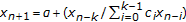
Here, the stability of equilibrium points of the fractional difference equation

(1.1)

with the initial condition

(1.2)

is investigated. Here , , , , are known constants. Equation (1.1) generalizes a lot of different particular cases that are considered in [1–8, 16, 18, 19, 20, 22, 23, 24, 32, 35, 37].

Put

(1.3)

and suppose that (1.1) has some point of equilibrium (not necessary a positive one). Then by assumption

(1.4)

the equilibrium point is defined by the algebraic equation

(1.5)

By condition (1.4), equation (1.5) can be transformed to the form

(1.6)

It is clear that if

(1.7)

then (1.1) has two points of equilibrium

(1.8)

(1.9)

If

(1.10)

then (1.1) has only one point of equilibrium

(1.11)

And at last if

(1.12)

then (1.1) has not equilibrium points.

Remark 1.1.

Consider the case , . From (1.5) we obtain the following. If and , then (1.1) has two points of equilibrium:

(1.13)

If and , then (1.1) has only one point of equilibrium: . If , then (1.1) has only one point of equilibrium: .

Remark 1.2.

Consider the case , . If , then (1.1) has only one point of equilibrium: . If , then each solution is an equilibrium point of (1.1).

2. Stochastic Perturbations, Centering, and Linearization—Definitions and Auxiliary Statements

Let be a probability space and let be a nondecreasing family of sub--algebras of , that is, for , let be the expectation, let , , be a sequence of -adapted mutually independent random variables such that , .

As it was proposed in [39, 40] and used later in [41–43] we will suppose that (1.1) is exposed to stochastic perturbations which are directly proportional to the deviation of the state of system (1.1) from the equilibrium point . So, (1.1) takes the form

(2.1)

Note that the equilibrium point of (1.1) is also the equilibrium point of (2.1).

Putting we will center (2.1) in the neighborhood of the point of equilibrium . From (2.1) it follows that

(2.2)

It is clear that the stability of the trivial solution of (2.2) is equivalent to the stability of the equilibrium point of (2.1).

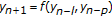
Together with nonlinear equation (2.2) we will consider and its linear part

(2.3)

Two following definitions for stability are used below.

Definition 2.1.

The trivial solution of (2.2) is called stable in probability if for any and there exists such that the solution satisfies the condition for any initial function such that .

Definition 2.2.

The trivial solution of (2.3) is called mean square stable if for any there exists such that the solution satisfies the condition for any initial function such that . If, besides, , for any initial function , then the trivial solution of (2.3) is called asymptotically mean square stable.

The following method for stability investigation is used below. Conditions for asymptotic mean square stability of the trivial solution of constructed linear equation (2.3) were obtained via V. Kolmanovskii and L. Shaikhet general method of Lyapunov functionals construction [44–46]. Since the order of nonlinearity of (2.2) is more than 1, then obtained stability conditions at the same time are [47–49] conditions for stability in the probability of the trivial solution of nonlinear equation (2.2) and therefore for stability in probability of the equilibrium point of (2.1).

Lemma 2.3.

(see [44]). If

(2.4)

then the trivial solution of (2.3) is asymptotically mean square stable.

Put

(2.5)

Lemma 2.4.

(see [44]). If

(2.6)

then the trivial solution of (2.3) is asymptotically mean square stable.

Consider also the necessary and sufficient condition for asymptotic mean square stability of the trivial solution of (2.3).

Let and be two square matrices of dimension such that has all zero elements except for and

(2.7)

Lemma 2.5 ([46]).

Let the matrix equation

(2.8)

has a positively semidefinite solution with . Then the trivial solution of (2.3) is asymptotically mean square stable if and only if

(2.9)

Corollary 2.6.

For condition (2.9) takes the form

(2.10)

(2.11)

If, in particular, , then condition (2.10) is the necessary and sufficient condition for asymptotic mean square stability of the trivial solution of (2.3) for .

Remark 2.7.

Put . If , then the trivial solution of (2.3) can be stable (e.g., or ), unstable (e.g., ) but cannot be asymptotically stable. Really, it is easy to see that if (in particular, ), then sufficient conditions (2.4) and (2.6) do not hold. Moreover, necessary and sufficient (for ) condition (2.10) does not hold too since if (2.10) holds, then we obtain a contradiction

(2.12)

Remark 2.8.

As it follows from results of [47–49] the conditions of Lemmas 2.3, 2.4, 2.5 at the same time are conditions for stability in probability of the equilibrium point of (2.1).

3. Stability of Equilibrium Points

From conditions (2.4), (2.6) it follows that . Let us check if this condition can be true for each equilibrium point.

Suppose at first that condition (1.7) holds. Then (2.1) has two points of equilibrium and defined by (1.8) and (1.9) accordingly. Putting via (2.5), (2.3), (1.3), we obtain that corresponding and are

(3.1)

So, . It means that the condition holds only for one from the equilibrium points and . Namely, if , then ; if , then ; if , then . In particular, if , then via Remark 1.1 and (2.3) we have , . Therefore, if , if , if .

So, via Remark 2.7, we obtain that equilibrium points and can be stable concurrently only if corresponding and are negative concurrently.

Suppose now that condition (1.10) holds. Then (2.1) has only one point of equilibrium (1.11). From (2.5), (2.3), (1.3), (1.11) it follows that corresponding equals

(3.2)

As it follows from Remark 2.7 this point of equilibrium cannot be asymptotically stable.

Corollary 3.1.

Let be an equilibrium point of (2.1) such that

(3.3)

Then the equilibrium point is stable in probability.

The proof follows from (2.3), Lemma 2.3, and Remark 2.8.

Corollary 3.2.

Let be an equilibrium point of (2.1) such that

(3.4)

(3.5)

Then the equilibrium point is stable in probability.

Proof.

Via (1.3), (2.3), (2.5) we have

(3.6)

Rewrite (2.6) in the form

(3.7)

and show that it holds. From (3.4) it follows that . Via we have

(3.8)

So,

(3.9)

It means that the condition of Lemma 2.4 holds. Via Remark 2.8 the proof is completed.

Corollary 3.3.

An equilibrium point of the equation

(3.10)

is stable in probability if and only if

(3.11)

(3.12)

The proof follows from (2.3), (2.10), (2.11).

4. Examples

Example 4.1.

Consider (3.10) with , , . From (1.3) and (1.7)–(1.9) it follows that , and for any fixed and such that equation (3.10) has two points of equilibrium

(4.1)

In Figure 1, the region where the points of equilibrium are absent (white region), the region where both points of equilibrium and are there but unstable (yellow region), the region where the point of equilibrium is stable only (red region), the region where the point of equilibrium is stable only (green region), and the region where both points of equilibrium and are stable (cyan region) are shown in the space of (). All regions are obtained via condition (3.11) for . In Figures 2, 3 one can see similar regions for and , accordingly, that were obtained via conditions (3.11), (3.12). In Figure 4 it is shown that sufficient conditions (3.3) and (3.4), (3.5) are enough close to necessary and sufficient conditions (3.11), (3.12): inside of the region where the point of equilibrium is stable (red region) one can see the regions of stability of the point of equilibrium that were obtained by condition (3.3) (grey and green regions) and by conditions (3.4), (3.5) (cyan and green regions). Stability regions obtained via both sufficient conditions of stability (3.3) and (3.4), (3.5) give together almost whole stability region obtained via necessary and sufficient stability conditions (3.11), (3.12).

Consider now the behavior of solutions of (3.10) with in the points , , , of the space of () (Figure 1). In the point with , both equilibrium points and are unstable. In Figure 5 two trajectories of solutions of (3.10) are shown with the initial conditions , , and , . In Figure 6 two trajectories of solutions of (3.10) with the initial conditions , , and , are shown in the point with , . One can see that the equilibrium point is stable and the equilibrium point is unstable. In the point with , the equilibrium point is unstable and the equilibrium point is stable. Two corresponding trajectories of solutions are shown in Figure 7 with the initial conditions , , and , . In the point with , both equilibrium points and are stable. Two corresponding trajectories of solutions are shown in Figure 8 with the initial conditions , , and , . As it was noted above in this case, corresponding and are negative: and .

Figure 1

Stability regions, .

Figure 2

Stability regions, .

Figure 3

Stability regions, .

Figure 4

Stability regions, .

Figure 5

Unstable equilibrium points and for , .

Figure 6

Stable equilibrium point and unstable for , .

Figure 7

Unstable equilibrium point and stable for , .

Figure 8

Stable equilibrium points and for , .

Example 4.2.

Consider the difference equation

(4.2)

Different particular cases of this equation were considered in [2–5, 16, 22, 23, 37].

Equation (4.2) is a particular case of (2.1) with

(4.3)

Suppose firstly that and consider two cases: (1) , (2) . In the first case,

(4.4)

In the second case,

(4.5)

In both cases, Corollary 3.1 gives stability condition in the form or

(4.6)

with

(4.7)

Corollary 3.2 in both cases gives stability condition in the form or (4.6) with

(4.8)

Since then condition (4.6), (4.7) is better than (4.6), (4.8).

In the case , Corollary 3.3 gives stability condition in the form

(4.9)

or

(4.10)

In particular, from (4.10) it follows that for , (this case was considered in [3, 23]) the equilibrium point is stable if and only if . Note that in [3] for this case the condition only is obtained.

In Figure 9 four trajectories of solutions of (4.2) in the case , , , are shown: (1) , , , (red line, stable solution); (2) , , , (brown line, unstable solution); (3) , , , (blue line, unstable solution); (4) , , , (green line, stable solution).

In the case , , Corollary 3.3 gives stability condition in the form

(4.11)

or

(4.12)

For example, from (4.12) it follows that for , (this case was considered in [22, 37]), the equilibrium point is stable if and only if . In Figure 10 four trajectories of solutions of (4.2) in the case , , , are shown: (1) , , , (red line, stable solution); (2) , , , (brown line, unstable solution); (3) , , , (blue line, unstable solution); (4) , , , (green line, stable solution).

Via simulation of a sequence of mutually independent random variables consider the behavior of the equilibrium point by stochastic perturbations. In Figure 11 one thousand trajectories are shown for , , , , . In this case, stability condition (4.12) holds () and therefore the equilibrium point is stable: all trajectories go to . Putting , we obtain that stability condition (4.12) does not hold (). Therefore, the equilibrium point is unstable: in Figure 12 one can see that 1000 trajectories fill the whole space.

Note also that if goes to zero all obtained stability conditions are violated. Therefore, by conditions the equilibrium point is unstable.

Figure 9

Stable equilibrium points and , unstable and .

Figure 10

Stable equilibrium points and , unstable and .

Figure 11

Stable equilibrium point for , , .

Figure 12

Unstable equilibrium point for , , .

Example 4.3.

Consider the equation

(4.13)

(its particular cases were considered in [18, 19, 35]). Equation (4.13) is a particular case of (2.1) with , , , . From (1.7)–(1.9) it follows that by condition it has two equilibrium points

(4.14)

For equilibrium point sufficient conditions (3.3) and (3.4), (3.5) give

(4.15)

From (3.11), (3.12) it follows that an equilibrium point of (4.13) is stable in probability if and only if

(4.16)

For example, for from (4.15) we obtain

(4.17)

From (4.16) it follows

(4.18)

Similar for from (4.15) we obtain

(4.19)

From (4.16) it follows

(4.20)

Put, for example, . Then (4.13) has two equilibrium points: , . From (4.15)-(4.16) it follows that the equilibrium point is unstable and the equilibrium point is stable in probability if and only if

(4.21)

Note that for particular case , , , in [35] it is shown that the equilibrium point is locally asymptotically stable if ; and for particular case , , , in [18] it is shown that the equilibrium point is locally asymptotically stable if . It is easy to see that both these conditions follow from (4.21).

Similar results can be obtained for the equation that was considered in [1].

In Figure 13 one thousand trajectories of (4.13) are shown for , , , , , . In this case stability condition (4.21) holds () and therefore the equilibrium point is stable: all trajectories go to zero. Putting , we obtain that stability condition (4.21) does not hold (). Therefore, the equilibrium point is unstable: in Figure 14 one can see that 1000 trajectories by the initial condition , fill the whole space.

Figure 13

Stable equilibrium point for , , , .

Figure 14

Unstable equilibrium point for , , , .

Example 4.4.

Consider the equation

(4.22)

that is a particular case of (3.10) with , , , , , . As it follows from (1.4), (1.7)–(1.9) by conditions , , (4.22) has two equilibrium points

(4.23)

From (3.11), (3.12) it follows that an equilibrium point of (4.22) is stable in probability if and only if

(4.24)

Substituting (4.23) into (4.24), we obtain stability conditions immediately in the terms of the parameters of considered equation (4.22): the equilibrium point is stable in probability if and only if

(4.25)

the equilibrium point is stable in probability if and only if

(4.26)

Note that in [24] equation (4.18) was considered with and positive , . There it was shown that equilibrium point is locally asymptotically stable if and only if that is a part of conditions (4.25).

In Figure 15 the region where the points of equilibrium are absent (white region), the region where the both points of equilibrium and are there but unstable (yellow region), the region where the point of equilibrium is stable only (red region), the region where the point of equilibrium is stable only (green region) and the region where the both points of equilibrium and are stable (cyan region) are shown in the space of (,). All regions are obtained via conditions (4.25), (4.26) for . In Figures 16 similar regions are shown for .

Consider the point (Figure 15) with , . In this point both equilibrium points and are unstable. In Figure 17 two trajectories of solutions of (4.22) are shown with the initial conditions , and , . In Figure 18 two trajectories of solutions of (4.22) with the initial conditions , and , are shown in the point (Figure 15) with . One can see that the equilibrium point is stable and the equilibrium point is unstable. In the point (Figure 15) with , the equilibrium point is unstable and the equilibrium point is stable. Two corresponding trajectories of solutions are shown in Figure 19 with the initial conditions and , . In the point (Figure 15) with , both equilibrium points and are stable. Two corresponding trajectories of solutions are shown in Figure 20 with the initial conditions , and , .

Consider the behavior of the equilibrium points of (4.22) by stochastic perturbations with . In Figure 21 trajectories of solutions are shown for , (the point in Figure 16) with the initial conditions , and . One can see that the equilibrium point (red trajectories) is stable and the equilibrium point (green trajectories) is unstable. In Figure 22 trajectories of solutions are shown for , (the point in Figure 16) with the initial conditions , and , . In this case both equilibrium points (red trajectories) and (green trajectories) are stable.

Figure 15

Stability regions, .

Figure 16

Stability regions, .

Figure 17

Unstable equilibrium points and for , .

Figure 18

Stable equilibrium point and unstable for , .

Figure 19

Unstable equilibrium point and stable for , .

Figure 20

Stable equilibrium points and for , .

Figure 21

Stable equilibrium points and for , , .

Figure 22

Stable equilibrium points and for , , .

References

Aboutaleb MT, El-Sayed MA, Hamza AE:Stability of the recursive sequence
. Journal of Mathematical Analysis and Applications 2001, 261(1):126-133. 10.1006/jmaa.2001.7481
Abu-Saris RM, DeVault R:Global stability of
. Applied Mathematics Letters 2003, 16(2):173-178. 10.1016/S0893-9659(03)80028-9
Amleh AM, Grove EA, Ladas G, Georgiou DA:On the recursive sequence
. Journal of Mathematical Analysis and Applications 1999, 233(2):790-798. 10.1006/jmaa.1999.6346
Berenhaut KS, Foley JD, Stević S:Quantitative bounds for the recursive sequence
. Applied Mathematics Letters 2006, 19(9):983-989. 10.1016/j.aml.2005.09.009
Berenhaut KS, Foley JD, Stević S:The global attractivity of the rational difference equation
. Proceedings of the American Mathematical Society 2007, 135(4):1133-1140. 10.1090/S0002-9939-06-08580-7
Berenhaut KS, Stević S:The difference equation
has solutions converging to zero. Journal of Mathematical Analysis and Applications 2007, 326(2):1466-1471. 10.1016/j.jmaa.2006.02.088
Camouzis E, Chatterjee E, Ladas G:On the dynamics of
. Journal of Mathematical Analysis and Applications 2007, 331(1):230-239. 10.1016/j.jmaa.2006.08.088
Camouzis E, Ladas G, Voulov HD:On the dynamics of
. Journal of Difference Equations and Applications 2003, 9(8):731-738. 10.1080/1023619021000042153
Camouzis E, Papaschinopoulos G:Global asymptotic behavior of positive solutions on the system of rational difference equations
,
,  . Applied Mathematics Letters 2004, 17(6):733-737. 10.1016/S0893-9659(04)90113-9
Çinar C:On the difference equation
. Applied Mathematics and Computation 2004, 158(3):813-816. 10.1016/j.amc.2003.08.122
Çinar C:On the positive solutions of the difference equation
. Applied Mathematics and Computation 2004, 156(2):587-590. 10.1016/j.amc.2003.08.010
Çinar C:On the positive solutions of the difference equation system
,  . Applied Mathematics and Computation 2004, 158(2):303-305. 10.1016/j.amc.2003.08.073
. Applied Mathematics and Computation 2004, 150(1):21-24. 10.1016/S0096-3003(03)00194-2
Clark D, Kulenović MRS: A coupled system of rational difference equations. Computers & Mathematics with Applications 2002, 43(6-7):849-867. 10.1016/S0898-1221(01)00326-1
Clark CA, Kulenović MRS, Selgrade JF: On a system of rational difference equations. Journal of Difference Equations and Applications 2005, 11(7):565-580. 10.1080/10236190412331334464
DeVault R, Kent C, Kosmala W:On the recursive sequence
. Journal of Difference Equations and Applications 2003, 9(8):721-730. 10.1080/1023619021000042162
Elabbasy EM, El-Metwally H, Elsayed EM:On the difference equation
. Advances in Difference Equations 2006, 2006:-10.
El-Owaidy HM, Ahmed AM, Mousa MS:On the recursive sequences
. Applied Mathematics and Computation 2003, 145(2-3):747-753. 10.1016/S0096-3003(03)00271-6
Gibbons CH, Kulenovic MRS, Ladas G:On the recursive sequence
. Mathematical Sciences Research Hot-Line 2000, 4(2):1-11.
Gibbons CH, Kulenović MRS, Ladas G, Voulov HD:On the trichotomy character of
. Journal of Difference Equations and Applications 2002, 8(1):75-92. 10.1080/10236190211940
Grove EA, Ladas G, McGrath LC, Teixeira CT: Existence and behavior of solutions of a rational system. Communications on Applied Nonlinear Analysis 2001, 8(1):1-25.
Gutnik L, Stević S: On the behaviour of the solutions of a second-order difference equation. Discrete Dynamics in Nature and Society 2007, 2007:-14.
Hamza AE:On the recursive sequence
. Journal of Mathematical Analysis and Applications 2006, 322(2):668-674. 10.1016/j.jmaa.2005.09.029
Kosmala WA, Kulenović MRS, Ladas G, Teixeira CT:On the recursive sequence
. Journal of Mathematical Analysis and Applications 2000, 251(2):571-586. 10.1006/jmaa.2000.7032
Kulenović MRS, Ladas G: Dynamics of Second Order Rational Difference Equations: With Open Problems and Conjectures. Chapman & Hall/CRC, Boca Raton, Fla, USA; 2001:xii+218.
Kulenović MRS, Nurkanović M: Asymptotic behavior of a competitive system of linear fractional difference equations. Advances in Difference Equations 2006, 2006:-13.
Kulenović MRS, Nurkanović M: Asymptotic behavior of a two dimensional linear fractional system of difference equations. Radovi Matematički 2002, 11(1):59-78.
Kulenović MRS, Nurkanović M: Asymptotic behavior of a system of linear fractional difference equations. Journal of Inequalities and Applications 2005, 2005(2):127-143.
Li X: Global behavior for a fourth-order rational difference equation. Journal of Mathematical Analysis and Applications 2005, 312(2):555-563. 10.1016/j.jmaa.2005.03.097
Li X: Qualitative properties for a fourth-order rational difference equation. Journal of Mathematical Analysis and Applications 2005, 311(1):103-111. 10.1016/j.jmaa.2005.02.063
Papaschinopoulos G, Schinas CJ:On the system of two nonlinear difference equations
,  . International Journal of Mathematics and Mathematical Sciences 2000, 23(12):839-848. 10.1155/S0161171200003227
Stević S:On the recursive sequence
. Discrete Dynamics in Nature and Society 2007, 2007:-7.
Sun T, Xi H:On the system of rational difference equations
,  . Advances in Difference Equations 2006, 2006:-8.
Sun T, Xi H, Hong L:On the system of rational difference equations
,  . Advances in Difference Equations 2006, 2006:-7.
Sun T, Xi H, Wu H:On boundedness of the solutions of the difference equation
. Discrete Dynamics in Nature and Society 2006, 2006:-7.
Xi H, Sun T: Global behavior of a higher-order rational difference equation. Advances in Difference Equations 2006, 2006:-7.
Yan X-X, Li W-T, Zhao Z:On the recursive sequence
. Journal of Applied Mathematics & Computing 2005, 17(1-2):269-282. 10.1007/BF02936054
Yang X:On the system of rational difference equations
,  . Journal of Mathematical Analysis and Applications 2005, 307(1):305-311. 10.1016/j.jmaa.2004.10.045
Beretta E, Kolmanovskii V, Shaikhet L: Stability of epidemic model with time delays influenced by stochastic perturbations. Mathematics and Computers in Simulation 1998, 45(3-4):269-277. 10.1016/S0378-4754(97)00106-7
Shaikhet L: Stability of predator-prey model with aftereffect by stochastic perturbation. Stability and Control: Theory and Applications 1998, 1(1):3-13.
Bandyopadhyay M, Chattopadhyay J: Ratio-dependent predator-prey model: effect of environmental fluctuation and stability. Nonlinearity 2005, 18(2):913-936. 10.1088/0951-7715/18/2/022
Bradul N, Shaikhet L: Stability of the positive point of equilibrium of Nicholson's blowflies equation with stochastic perturbations: numerical analysis. Discrete Dynamics in Nature and Society 2007, 2007:-25.
Carletti M: On the stability properties of a stochastic model for phage-bacteria interaction in open marine environment. Mathematical Biosciences 2002, 175(2):117-131. 10.1016/S0025-5564(01)00089-X
Kolmanovskii V, Shaikhet L: General method of Lyapunov functionals construction for stability investigation of stochastic difference equations. In Dynamical Systems and Applications, World Scientific Series in Applicable Analysis. Volume 4. World Science, River Edge, NJ, USA; 1995:397-439.
Kolmanovskii V, Shaikhet L: Construction of Lyapunov functionals for stochastic hereditary systems: a survey of some recent results. Mathematical and Computer Modelling 2002, 36(6):691-716. 10.1016/S0895-7177(02)00168-1
Shaikhet L: Necessary and sufficient conditions of asymptotic mean square stability for stochastic linear difference equations. Applied Mathematics Letters 1997, 10(3):111-115. 10.1016/S0893-9659(97)00045-1
Paternoster B, Shaikhet L: About stability of nonlinear stochastic difference equations. Applied Mathematics Letters 2000, 13(5):27-32. 10.1016/S0893-9659(00)00029-X
Shaikhet L: Stability in probability of nonlinear stochastic systems with delay. Matematicheskie Zametki 1995, 57(1):142-146.
Shaikhet L: Stability in probability of nonlinear stochastic hereditary systems. Dynamic Systems and Applications 1995, 4(2):199-204.
Author information
Authors and Affiliations
Corresponding author
Rights and permissions
Open Access This article is distributed under the terms of the Creative Commons Attribution 2.0 International License (https://creativecommons.org/licenses/by/2.0), which permits unrestricted use, distribution, and reproduction in any medium, provided the original work is properly cited.
About this article
Cite this article
Paternoster, B., Shaikhet, L. Stability of Equilibrium Points of Fractional Difference Equations with Stochastic Perturbations. Adv Differ Equ 2008, 718408 (2008). https://doi.org/10.1155/2008/718408
Received:
Accepted:
Published:
DOI: https://doi.org/10.1155/2008/718408