Asymptotic Representation of the Solutions of Linear Volterra Difference Equations

Abstract

This article analyses the asymptotic behaviour of solutions of linear Volterra difference equations. Some sufficient conditions are presented under which the solutions to a general linear equation converge to limits, which are given by a limit formula. This result is then used to obtain the exact asymptotic representation of the solutions of a class of convolution scalar difference equations, which have real characteristic roots. We give examples showing the accuracy of our results.

1. Introduction

The literature on the asymptotic theory of the solutions of Volterra difference equations is extensive, and application of this theory is rapidly increasing to various fields. For the basic theory of difference equations, we choose to refer to the books by Agarwal [1], Elaydi [2], and Kelley and Peterson [3]. Recent contribution to the asymptotic theory of difference equations is given in the papers by Kolmanovskii et al. [4], Medina [5], Medina and Gil [6], and Song and Baker [7]; see [8–19] for related results.

The results obtained in this paper are motivated by the results of two papers by Applelby et al. [20], and Philos and Purnaras [21].

This paper studies the asymptotic constancy of the solution of the system of nonconvolution Volterra difference equation

(1.1)

with the initial condition

(1.2)

where , and are sequences with elements in and , respectively.

Under appropriate assumptions, it is proved that the solution converges to a finite limit which obeys a limit formula. Our paper develops further the recent work [20]. The distinction between the works is explained as follows. For large enough , in fact , the sum in (1.1) can be split into three terms

(1.3)

since

(1.4)

In [20, Theorem 3.1] the middle sum in (1.3) contributed nothing to the limit , since it was assumed that

(1.5)

In our case, we split the sum in (1.1) only into two terms, and the condition (1.5) is not assumed. In fact, we show an example in Section 4, where (1.5) does not hold and hence in [20, Theorem 3.1] is not applicable. At the same time our main theorem gives a limit formula. It is also interesting to note that our proof is simpler than it was applied in [20].

Once our main result for, the general equation, (1.1) has been proven, we may use it for the scalar convolution Volterra difference equation with infinite delay,

(1.6)

with the initial condition,

(1.7)

where , and and are real sequences.

Here, denotes the forward difference operator to be defined as usual, that is, .

If we look for a solution of the homogeneous equation associated with (1.6), we see that is a root of the characteristic equation

(1.8)

We immediately observe that is a simple root if

(1.9)

In the paper [21] (see also [22]), it is shown that if satisfies (1.8) and (1.9), and the initial sequence is suitable, then for the solution of (1.6) and (1.7) the sequence , is bounded. Furthermore, some extra conditions guarantee that the limit is finite and satisfies a limit formula.

In our paper, we improve considerably the result in [21]. First, we give explicit necessary and sufficient conditions for the existence of a for which (1.8) and (1.9) are satisfied. Second, we prove the existence of the limit and give a limit formula for under the condition only . These two statements are formulated in our second main theorem stated in Section 3. The proof of the existence of is based on our first main result.

The article is organized as follows. In Section 2, we briefly explain some notation and definitions which are used to state and to prove our results. In Section 3, we state our two main results, whose proofs are relegated to Section 5.

Our theory is illustrated by examples in Section 4, including an interesting nonconvolution equation. This example shows the significance of the middle sum in (1.3), since only this term contributes to the limit of the solution of (1.1) in this case.

2. Mathematical Preliminaries

In this section, we briefly explain some notation and well-known mathematical facts which are used in this paper.

Let be the set of integers, and . stands for the set of all -dimensional column vectors with real components and is the space of all by real matrices. The zero matrix in is denoted by , and the identity matrix by . Let be the matrix in whose elements are all . The absolute value of the vector and the matrix is defined by and , respectively. The vector and the matrix is nonnegative if and , , respectively. In this case, we write and . can be endowed with any norms, but they are equivalent. A vector norm is denoted by and the norm of a matrix in induced by this vector norm is also denoted by . The spectral radius of the matrix is given by , which is independent of the norm employed to calculate it.

A partial ordering is defined on by letting if and only if . The partial ordering enables us to define the , and so forth for the sequences of vectors and matrices, which can also be determined componentwise and elementwise, respectively. It is known that for , and if and .

3. The Main Results

First, consider the nonconvolutional linear Volterra difference equation

(3.1)

with initial condition

(3.2)

Here, we assume

• (H1) and are sequences with elements in and , respectively;

• (H2) for any fixed the limit is finite and ;

• (H3) the matrix

  

  (3.3)

  is finite;

• (H4) the matrix

  

  (3.4)

  is finite and ;

• (H5) the limit is finite.

By a solution of (3.1), we mean a sequence in satisfying (3.1) for any . It is clear that (3.1) with initial condition (3.2) has a unique solution.

Now, we are in a position to state our first main result.

Theorem 3.1.

Assume (H₁)–(H₅) are satisfied. Then for any the unique solution of (3.1) and (3.2) has a finite limit at and it satisfies

(3.5)

Under conditions and

(3.6)

and hence yields , thus is invertible. On the other hand under our conditions the unique solution of (3.1) and (3.2) is a bounded sequence, therefore is finite, and (3.5) makes sense.

The second main result is dealing with the scalar Volterra difference equation

(3.7)

with the initial condition

(3.8)

where , and are given.

By a solution of the Volterra difference equation (3.7) we mean a sequence satisfies (3.7) for any .

In what follows, by we will denote the set of all initial sequence such that for each

(3.9)

exists.

It can be easily seen that for any initial sequence , (3.7) has exactly one solution satisfying (3.8). This unique solution is denoted by and it is called the solution of the initial value problem (3.7), (3.8).

The asymptotic representation of the solutions of (3.7) is given under the next condition.

• (A) There exists a for which

  

  (3.10)
  

  (3.11)

  From the theory of the infinite series, one can easily see that condition (A) yields

  

  (3.12)

is finite. Moreover, the mapping defined by

(3.13)

is real valued on . It is also clear (see Section 5) that if there is an such that , and if then the equation

(3.14)

has a unique solution, say .

Now we formulate the following more explicit condition:

• (B) either , , and

  

  (3.15)

  or there is an with , and

  • (i) defined in (3.12) is finite,

  • (ii) if , then the constant satisfies either

    

    (3.16)

    or

    

    (3.17)

  • (iii) if , then the constant satisfies either

    

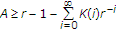    (3.18)

    or

    

    (3.19)

Remark 3.2.

Let be a sequence such that for some . It will be proved in Lemma 5.7 that there is at most one satisfying (3.10) and (3.11). It is an easy consequence of this statement that if satisfies (3.10) and (3.11), and is a solution of (3.10), then , thus is the leading root of (3.10). Really, from the condition we have

(3.20)

that is (3.11) holds for instead of , and this contradicts the uniqueness of .

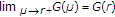
Now, we are ready to state our second result which will be proved in Section 5. This result shows that the implicit condition (A) and the explicit condition (B) are equivalent and the solutions of (3.7) can be asymptotically characterized by as .

Theorem 3.3.

Let , and be given. Then

Condition (A) holds if and only if condition (B) is satisfied.

If condition (A) or equivalently condition (B) holds, moreover

(3.21)

is finite, then for the solution of (3.7), (3.8) the limit is finite and it obeys

(3.22)

4. Examples and the Discussion of the Results

In this section, we illustrate our results by examples and the interested reader could also find some discussions.

Example 4.1.

Our Theorem 3.1 is given for system of equations, however the next example shows that this result is also new even in scalar case.

Let us consider the scalar nonconvolution Volterra difference equation

(4.1)

with the initial condition

(4.2)

where and real, and is a real sequence such that its limit is finite.

Now, let the values and the sequence be defined by

(4.3)

Then, it can be easily seen that problem (4.1), (4.2) is equivalent to problem (3.1), (3.2).

We find that for any fixed .

It is known that

(4.4)

where is the well-known Beta function at defined by

(4.5)

Using the nonnegativity of , and Lemma 5.2 we have that

(4.6)

Now, one can easily see that for the sequences and all of the conditions of Theorem 3.1 are satisfied. Thus, by Theorem 3.1 we get that the solution of the initial value problem (4.1), (4.2) satisfies

(4.7)

On the other hand, we know (see [23]) that

(4.8)

and hence in [20, Theorem 3.1] is not applicable.

Example 4.2.

Let and be given integers, and assume if and if . Then,

(4.9)

Thus, (3.7) reduces to the delay difference equation

(4.10)

and for any sequence holds.

Since for any large enough , , moreover the function defined in (3.13) satisfies

(4.11)

Let be the unique value satisfying

(4.12)

Now, statement() of Theorem 3.3 is applicable and so the next statement is valid.

Proposition 4.3.

For an there is a such that

(4.13)

hold if and only if either

(4.14)

or

(4.15)

is satisfied.

Now, let and . Then , moreover (4.14) and (4.15) reduce to

(4.16)

If especially and , then , moreover (4.14) and (4.15) are equivalent to the condition

(4.17)

Example 4.4.

Let and . Then, (3.7) has the following form:

(4.18)

It is clear that , and the function defined in (3.13) is given by

(4.19)

moreover is the unique positive root of .

Thus statement () in Theorem 3.3 is applicable and as a corollary of it we obtain the following.

Proposition 4.5.

There is a such that (3.10) and (3.11) hold with the sequence , , if and only if either

(4.20)

or

(4.21)

Example 4.6.

Let and let , . Here is the extended binomial coefficient, that is

(4.22)

In this case, and by using the well-known properties of the binomial series, we find

(4.23)

Thus, , therefore by statement () of Theorem 3.3 we get the following.

Proposition 4.7.

There is a such that (3.10) and (3.11) hold with the sequence , if and only if either

(4.24)

or

(4.25)

where is the unique positive solution of the equation

(4.26)

Example 4.8.

Let and , and . Then, (3.7) reduces to the special form

(4.27)

It is not difficult to see that ,

(4.28)

and . From statement of Theorem 3.3 we have the following.

Proposition 4.9.

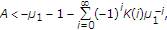
There is a such that (3.10) and (3.11) hold with the sequence , if and only if either

(4.29)

or

(4.30)

where is the well-known Riemann function.

5. Proofs of the Main Theorems

5.1. Proof of Theorem 3.1

To prove Theorem 3.1 we need the next result from [20].

Theorem A.

Let us consider the initial value problem ( 3.1 ), ( 3.2 ). Suppose that there are such that

(5.1)

(5.2)

Assume also that. Then, there is a nonnegative matrix, independent of and , such that the solutionof ( 3.1 ), ( 3.2 ) satisfies

(5.3)

Now, we prove some lemmas.

Lemma 5.1.

The hypotheses of Theorem 3.1 imply that the hypotheses of Theorem A are satisfied, and hence the solution of (3.1), (3.2) is bounded.

Proof.

Let be such that . This can be satisfied because . Then, there is an for which

(5.4)

and hence for an , we have

(5.5)

Thus,

(5.6)

therefore,

(5.7)

But the matrices are nonnegative in the above inequality, thus

(5.8)

and this shows (5.1). Since condition holds, we get

(5.9)

therefore,

(5.10)

thus (5.2) is satisfied.

In the next lemma we give an equivalent form of .

Lemma 5.2.

Let be a sequence of real by matrices which satisfies . Then, there exists a real by matrix such that

(5.11)

if and only if

(5.12)

is finite. In both cases

(5.13)

If satisfies too, and (5.11) holds, then .

Proof.

First we show that

(5.14)

is finite if and only if

(5.15)

is finite, and in both cases

(5.16)

These come from , since

(5.17)

Suppose is a real by matrix. Then, by for every

(5.18)

and hence

(5.19)

Now, suppose that (5.11) holds. Then by (5.19), either

(5.20)

or

(5.21)

Both of the previous cases implies that

(5.22)

which shows that

(5.23)

is finite and

(5.24)

As we have seen, this is equivalent with (5.12). If (5.12) is true or equivalently

(5.25)

is finite, then by (5.19)

(5.26)

satisfies (5.11). follows from . The proof is now complete.

Lemma 5.3.

The hypotheses of Theorem 3.1 imply that

(5.27)

is the only vector satisfying the equation

(5.28)

Proof.

Since the matrix is invertible, which shows the uniqueness part of the lemma. On the other hand, by Lemma 5.1 we have that is a bounded sequence, and hence is finite. Thus, is well defined and satisfies (5.28). The proof is complete.

Lemma 5.4.

The vector defined by (5.27) satisfies the relation

(5.29)

for any , where the sequence , , satisfies

(5.30)

Proof.

Let be arbitrarily fixed and

(5.31)

But under the hypotheses of Theorem 3.1 we find

(5.32)

Now, by Lemma 5.2

(5.33)

and hence (5.30) holds. On the other hand, it can be easily seen that by the above definition of the relation (5.29) also holds. The proof is complete.

Now, we prove Theorem 3.1.

Proof.

Let be arbitrarily fixed. Then, (3.1) can be written in the form

(5.34)

Subtracting (5.29) from the above equation, we get

(5.35)

On the other hand, by Lemma 5.1, is bounded and hence

(5.36)

is finite. Let be arbitrarily fixed and . Then there is an such that

(5.37)

Thus, (5.35) yields

(5.38)

From this it follows:

(5.39)

Thus,

(5.40)

and hence Lemma 5.4 implies that

(5.41)

Since is a nonnegative matrix with , we have that . Thus,

(5.42)

and hence the proof of Theorem 3.1 is complete.

5.2. Proof of Theorem 3.3

Theorem 3.3 will be proved after some preparatory lemmas.

In the next lemma, we show that (3.7) can be transformed into an equation of the form (3.1) by using the transformation

(5.43)

Lemma 5.5.

Under the conditions of Theorem 3.3, the sequence defined by (5.43) satisfies (3.1), where the sequences and are defined by

(5.44)

(5.45)

Proof.

Let be defined by (5.43). Then,

(5.46)

Thus,

(5.47)

On the other hand, from (3.7) it follows:

(5.48)

Thus,

(5.49)

and hence

(5.50)

But

(5.51)

Therefore,

(5.52)

where is defined in (5.45). By interchanging the order of the summation we get

(5.53)

This and (5.52) yield

(5.54)

By using the definition , we have

(5.55)

and hence

(5.56)

But by using the definition of in (5.44) the proof of the lemma is complete.

In the next lemma, we collect some properties of the function defined in (3.13).

Lemma 5.6.

Let be a sequence such that for some and

(5.57)

Then, the function defined in (3.13) has the following properties.

• (a) The series of functions

  

  (5.58)

  is convergent on and it is divergent on .

• (b)
• (c)

• (d) is strictly decreasing.

• (e) If , then the equation has a unique solution.

Proof.

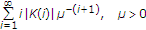
(a) The root test can be applied. (b) The series of functions (5.58) is uniformly convergent on for every , and this, together with , implies the result. (c) If is finite, then the series of functions (5.58) is uniformly convergent on , hence is continuous on . Suppose now that and . Let be fixed and let such that

(5.59)

Since

(5.60)

there is a such that

(5.61)

whenever , and this shows . Finally, we consider the case . Then, follows from the condition . (d) The series of functions (5.58) can be differentiated term-by-term within , and therefore , . Together with (c) this gives the claim. (e) We have only to apply (d), (c), and (b). The proof is complete.

We are now in a position to prove Theorem 3.3.

Proof.

(a) Let for all . Then, it is easy to see that there is a such that (3.10) holds if and only if (3.15) is true, and in this case (3.11) is also satisfied. Suppose for some . Let be finite. By the root test, the series

(5.62)

are convergent for all . Moreover, it can be easily verified that the series

(5.63)

are absolutely convergent, whenever is finite. Define the functions by

(5.64)

where if is finite and , otherwise. The series of functions in (5.64) are uniformly convergent on for every , hence and are continuous. Further,

(5.65)

Let if , and let if . It now follows from the previous inequalities and Lemma 5.6(d) that

(5.66)

and hence is strictly increasing on . It is immediate that . If (3.10) is hold for some , then the convergence of the series implies . Suppose . It is simple to see that there is a satisfying (3.10) if and only if either (in case ) or (in case ). Moreover, the existence of a satisfying (3.11) is equivalent to either (in case ) or (in case ). Now, the result follows from the properties of the functions . The proof of (a) is complete. (b) In virtue of Lemma 5.5 the proof of the theorem will be complete if we show that the sequences and satisfy the conditions (H₂)–(H₅) in Section 3. Since the series is convergent,

(5.67)

and hence . Thus holds. Now, let and consider . In fact

(5.68)

Thus,

(5.69)

Thus,

(5.70)

is finite and . In a similar way, one can easily prove that

(5.71)

is also finite. It is also clear that

(5.72)

is finite. Thus, by Theorem 3.1 we get that the limit

(5.73)

is finite and satisfies the required relation (3.22). The proof is now complete.

Lemma 5.7.

Let be a sequence such that for some . Then, there is at most one satisfying (3.10) and (3.11).

Proof.

Suppose on the contrary that there exist two different numbers from , denoted by and , such that (3.10) and (3.11) hold. Then,

(5.74)

(5.75)

It follows from (5.74), the mean value inequality and (5.75) that

(5.76)

and this is a contradiction.

References

Agarwal RP: Difference Equations and Inequalities: Theory, Methods, and Application, Monographs and Textbooks in Pure and Applied Mathematics. Volume 228. 2nd edition. Marcel Dekker, New York, NY, USA; 2000:xvi+971.
Elaydi S: An Introduction to Difference Equations, Undergraduate Texts in Mathematics. 3rd edition. Springer, New York, NY, USA; 2005:xxii+539.
Kelley WG, Peterson AC: Difference Equations: An Introduction with Applications. Academic Press, Boston, Mass, USA; 1991:xii+455.
Kolmanovskii VB, Castellanos-Velasco E, Torres-Muñoz JA: A survey: stability and boundedness of Volterra difference equations. Nonlinear Analysis: Theory, Methods & Applications 2003, 53(7-8):861-928. 10.1016/S0362-546X(03)00021-X
Medina R: Asymptotic behavior of Volterra difference equations. Computers & Mathematics with Applications 2001, 41(5-6):679-687. 10.1016/S0898-1221(00)00312-6
Medina R, Gil MI: The freezing method for abstract nonlinear difference equations. Journal of Mathematical Analysis and Applications 2007, 330(1):195-206. 10.1016/j.jmaa.2006.07.074
Song Y, Baker CTH: Admissibility for discrete Volterra equations. Journal of Difference Equations and Applications 2006, 12(5):433-457. 10.1080/10236190600563260
Agarwal RP, Pituk M: Asymptotic expansions for higher-order scalar difference equations. Advances in Difference Equations 2007, 2007:-12.
Berezansky L, Braverman E: On exponential dichotomy, Bohl-Perron type theorems and stability of difference equations. Journal of Mathematical Analysis and Applications 2005, 304(2):511-530. 10.1016/j.jmaa.2004.09.042
Bodine S, Lutz DA: Asymptotic solutions and error estimates for linear systems of difference and differential equations. Journal of Mathematical Analysis and Applications 2004, 290(1):343-362. 10.1016/j.jmaa.2003.09.068
Bodine S, Lutz DA: On asymptotic equivalence of perturbed linear systems of differential and difference equations. Journal of Mathematical Analysis and Applications 2007, 326(2):1174-1189. 10.1016/j.jmaa.2006.03.070
Driver RD, Ladas G, Vlahos PN: Asymptotic behavior of a linear delay difference equation. Proceedings of the American Mathematical Society 1992, 115(1):105-112. 10.1090/S0002-9939-1992-1111217-0
Elaydi S, Murakami S, Kamiyama E: Asymptotic equivalence for difference equations with infinite delay. Journal of Difference Equations and Applications 1999, 5(1):1-23. 10.1080/10236199908808167
Elaydi S: Asymptotics for linear difference equations. II. Applications. In New Trends in Difference Equations. Taylor & Francis, London, UK; 2002:111-133.
Graef JR, Qian C: Asymptotic behavior of a forced difference equation. Journal of Mathematical Analysis and Applications 1996, 203(2):388-400. 10.1006/jmaa.1996.0387
Győri I: Sharp conditions for existence of nontrivial invariant cones of nonnegative initial values of difference equations. Applied Mathematics and Computation 1990, 36(2):89-111. 10.1016/0096-3003(90)90014-T
Kolmanovskii V, Shaikhet L: Some conditions for boundedness of solutions of difference Volterra equations. Applied Mathematics Letters 2003, 16(6):857-862. 10.1016/S0893-9659(03)90008-5
Li ZH: The asymptotic estimates of solutions of difference equations. Journal of Mathematical Analysis and Applications 1983, 94(1):181-192. 10.1016/0022-247X(83)90012-4
Trench WF: Asymptotic behavior of solutions of Poincaré recurrence systems. Computers & Mathematics with Applications 1994, 28(1–3):317-324.
Applelby JAD, Győri I, Reynolds DW: On exact convergence rates for solutions of linear systems of Volterra difference equations. Journal of Difference Equations and Applications 2006, 12(12):1257-1275. 10.1080/10236190600986594
Philos ChG, Purnaras IK: The behavior of solutions of linear Volterra difference equations with infinite delay. Computers & Mathematics with Applications 2004, 47(10-11):1555-1563. 10.1016/j.camwa.2004.06.007
Philos ChG, Purnaras IK: On linear Volterra difference equations with infinite delay. Advances in Difference Equations 2006, 2006:-28.
Győri I, Horváth L: Limit theorems for discrete sums and convolutions. submitted
Acknowledgment
This work was supported by Hungarian National Foundation for Scientific Research Grant no. K73274.
Author information
Authors and Affiliations
Corresponding author
Rights and permissions
Open Access This article is distributed under the terms of the Creative Commons Attribution 2.0 International License (https://creativecommons.org/licenses/by/2.0), which permits unrestricted use, distribution, and reproduction in any medium, provided the original work is properly cited.
About this article
Cite this article
Győri, I., Horváth, L. Asymptotic Representation of the Solutions of Linear Volterra Difference Equations. Adv Differ Equ 2008, 932831 (2008). https://doi.org/10.1155/2008/932831
Received:
Accepted:
Published:
DOI: https://doi.org/10.1155/2008/932831