A Mixed Problem for Quasilinear Impulsive Hyperbolic Equations with Non Stationary Boundary and Transmission Conditions

Abstract

The initial-boundary value problem for a class of linear and nonlinear equations in Hilbert space is considers. We prove the existence and uniqueness of solution of this problem. The results of this investigation are applied to solvability of initial-boundary value problems for quasilinear impulsive hyperbolic equations with non-stationary transmission and boundary conditions.

1. Abstract Model Initial Boundary Value Problem with Non Stationary Boundary and Transmission Conditions for the Impulsive Linear Hyperbolic Equations

In paper [1] there is given an abstract scheme of investigation of mixed problems for hyperbolic equations with non stationary boundary conditions. In this direction, some results were obtained in [2].

In this paper, we offer the analogues abstract model of investigation of mixed problem with non stationary boundary and transmission conditions for impulsive linear and semilinear hyperbolic equations.

1.1. Statement of the Problem and Main Theorem

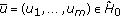
Let (; ; ; ) be Hilbert Spaces. Consider the following abstract initial-boundary value problem:

(1.1)

(1.2)

where , , , are the linear closed operators in ; are the linear operators from to ; are the linear operators from to ; are the linear operators from to; , , , .

We will investigate this problem under the following conditions.

• (i) Let , and let be densely in and continuously imbedded into it, .

In the Hilbert space , it was defined the system of the inner products , which generate uniform equivalent norms, that is,

(1.3)

For each , the function is continuously differentiable, .

In the Hilbert space , it was defined the system of the inner products , which generate uniform equivalent norms, that is,

(1.4)

For each , the function is continuously differentiable.

• (ii) For each and is a linear closed operator in whose domain is ; acts boundedly from to ; is strongly continuously differentiable.

• (iii) The linear operators , that act from to , bounded, where is interpolation space between and of order (see [3]).

• (iv) For each , the linear operators , that act from to , are bounded; is strongly continuously differentiable ,  ; .

• (v) The linear operators , from into , act boundedly , ; .

Let us introduce the following designations:

(1.5)

From condition (v), it follows that the space with the norm

(1.6)

is a subspace of

(1.7)

• (vi) Let the linear manifold be dense in , and let linear manifold be dense in .

• (vii) (Green's Identity). For arbitrary and , the following identity is valid:

(1.8)

• (viii) For all , the following inequality is fulfilled:

  

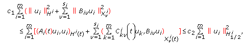  (1.9)

where .

• (ix) For each , an operator pencil

  

  (1.10)

which acts boundedly from to , has a regular point , where

(1.11)

• (x)
  

  (1.12)

• (xi) ,

(1.13)

Definition 1.1.

The function is called a solution of problem (1.1)-(1.2) if the function from to is continuous, and the function

(1.14)

from to is twice continuously differentiable and (1.1)-(1.2) are satisfied.

Theorem 1.2.

Let conditions (i)–(xi) are satisfied, then the problem (1.1)-(1.2) has a unique solution.

Proof.

We define the operator in the Hilbert space in the following way:

(1.15)

Then the problem (1.1)-(1.2) is represented as the Cauchy problem

(1.16)

where ,

(1.17)

It is obvious that if is the solution of problem (1.1)-(1.2), then is the solution of the problem (1.16). On the contrary, if

(1.18)

is the solution of problem (1.16), then , and is the solution of problem (1.1)-(1.2).

Let us define the system of inner product in Hilbert space in the following way:

(1.19)

where ,.

We denote space with inner product (1.19) by .

We will prove later the following auxiliary results.

Statement 1.3.

There exists such , that

(1.20)

and the function is continuously differentiable, where = .

Statement 1.4.

is a symmetric operator in for each .

Statement 1.5.

has a regular point for each in .

is symmetric and , for some ; therefore, for each is a selfadjoint operator in (see [4, chapter x]).

Taking into account (viii) and Statement 1.3, we get

(1.21)

that is, is a lower semibounded selfadjoint operator in .

Thus, the operator is selfadjoint and positive definite, where .

Problem (1.16) can be rewritten as

(1.22)

It is known that if and , then the problem (1.22) has a unique solution (see [5, 6]).

To complete the proof of the theorem, we need to show that and .

By conditions of the theorem ; , and are bounded operators from to . Therefore,

(1.23)

On the other hand, and , therefore, . Consequently,

(1.24)

From the definition of interpolation spaces (see [3, chapter 1], [7, chapter 1]), we get the following inclusion:

(1.25)

By virtue of definition, the powers of positive selfadjoint operator (see [8, chapter 2], [7, chapter 1]), we have that and

(1.26)

Assume that , then

(1.27)

By virtue of conditions (ii), (viii), (1.26), and (1.27), we get

(1.28)

Let . By virtue of condition (vi), is dense in ; therefore, there exists a sequence , such that and

(1.29)

Hence it follows, that

(1.30)

Then from (1.28) and (1.30) it follows that is fundamental in , that is,

(1.31)

where ,….

Thus, there exists such that

(1.32)

On the other hand, , therefore,

(1.33)

Hence,

(1.34)

where . From this, by virtue of (1.29), , that is,

(1.35)

Thus, . The theorem is proved.

1.2. Proof of Auxiliary Results

Validity of Statement 1.3 follows from condition (i), the Statement 1.4 from condition (vii).

Proof.

Consider in Hilbert space the equation

(1.36)

where .

Equation (1.36) is equivalent to the following system of differential-operator equations:

(1.37)

By virtue of (ix), problem (1.37) has a solution for some . Thus, for each ,

(1.38)

where is an identity operator in , that is, has a regular point.

2. Abstract Model of Initial Boundary Value Problem with Non Stationary Boundary and Transmission Conditions for the Impulsive Semilinear Hyperbolic Equations

Consider the following initial boundary value problem:

(2.1)

where , , , , , , , , and satisfy all conditions of Theorem 1.2.

Assume, that the nonlinear operators and satisfy the following conditions.

(xi′)Suppose that the nonlinear operators

(2.2)

satisfy the local Lipschitz conditions in the following sense: for arbitrary ,

(2.3)

where ,

(2.4)

Theorem 2.1.

Let conditions (i)–(x) and (xi′) be satisfied, then there exists , such that the problem (2.1) has a unique solution

(2.5)

Additionally, if

(2.6)

where , then . Otherwise, there exists , such that

(2.7)

In the Hilbert space , the problem (2.1) is represented as the Cauchy problem

(2.8)

where ,

(2.9)

From (), it follows that, for arbitrary ,

(2.10)

where .

Thus, the nonlinear operator satisfies the condition of local solvability of the Cauchy problem for the quasilinear hyperbolic equations in Hilbert space (see [6, 9]). Taking this into account, the problem (2.8) has a unique solution

(2.11)

3. Initial Boundary Value Problem with Non Stationary Boundary and Transmission Condition for the Impulsive Semilinear Hyperbolic Equations

Let . We consider in the domain the following mixed problem

(3.1)

where , , , are some functions, and are some functionals, which will be specified below, .

Recently, differential equations with impulses are great interest because of the needs of modern technology, where impulsive automatic control systems and impulsive computing systems are very important and intensively develop broadening the scope of their applications in technical problems, heterogeneous by their physical nature and functional purpose (see [10,chapter 1]).

Assume that the following conditions are held:

• (1⁰) ; , ,

• (2⁰) ,

• (3⁰) ,

• (4⁰) are nonlinear functionals acting from

  

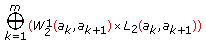  (3.2)

  to and for arbitrary the following inequality holds

  

  (3.3)

  where ,

  

  (3.4)

• (5⁰) are nonlinear functionals acting from

  

  (3.5)

  to and for arbitrary the following inequality holds

  

  (3.6)

  where , and —is defined as in (3.3),

• (6⁰) , , where

  

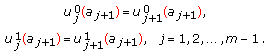  (3.7)

  By applying Theorem 2.1, we obtain the following result.

Theorem 3.1.

Let conditions (1⁰)–(6⁰) be held, then there exists a , such that the problem (3.1) has a unique solution , where

(3.8)

Proof.

Let us denote , , ,,  ,,,  , where ,.

In space and are defined the following inner products:

(3.9)

From differentiability of the functions , , and , it follows that the condition (i) is satisfied.

Let us define the following operators:

,

,

,

, for all other ,

,

,

, for all other ,

,

.

We also define the nonlinear operators as follows:

,

,

,

.

It is easy to verify that linear operators and the nonlinear operators , satisfy the conditions of Theorem 2.1, and the problem (3.1) is represented as an abstract initial boundary-value problem in the following way:

(3.10)

We will show that conditions of Theorem 2.1 are satisfied. Conditions (i)–(v) follow immediately from definitions of spaces and operators , and traces theorems (see [3, chapter 2]), where ; ; ; ; .

The linear manifolds and are defined in the following way:

(3.11)

We also define the spaces

(3.12)

Statement 3.2.

is dense in

(3.13)

Proof.

Assume that . Consider the following functions:

(3.14)

From definitions of , , we can see that

(3.15)

Let . Consider the function

(3.16)

It is obvious that . On the other hand, , where is a space of infinitely differentiable finite functions. Therefore, for an arbitrary , there exist the functions , , such that

(3.17)

By denoting from (3.17), we get

(3.18)

where .

Thus,

(3.19)

The following statement is proved in the same way.

Statement 3.3.

is dense .

Now, we prove that the condition (vi) holds.

Let , then

(3.20)

Similary, we obtain the following identity:

(3.21)

Thus, by virtue of (3.20)-(3.21), the condition (vi) holds.

From (3.20) or (3.21), putting , we also obtain the identity

(3.22)

that is, condition (viii) is satisfied, .

Now, we verify fulfillment of condition (ix). To that end, we consider the mixed problem

(3.23)

(3.24)

where ,; , , .

Let be the extend of function to . We consider the system of the differential equations

(3.25)

Hence, we have

(3.26)

where is a Fourier transformation of the function . From (3.26), we obtain , then functions satisfy (3.25), and their constrictions on () satisfy the (3.23). It is clear that . Considering linearity of the problem (3.23), (3.24), the solution can be represented in the form

(3.27)

where is a solution of the following problem:

(3.28)

(3.29)

where ,

(3.30)

A general solution of a system (3.28) is found in the following form:

(3.31)

Then, for determination of , from (3.29), we get the following system of the algebraic equations:

(3.32)

Let be a matrix of coefficients of system (3.32). From (3.32), it is clear that , where and as . Thus, for sufficiently large , is invertible and . Therefore, the system (3.32) has a unique solution.

Thus, for sufficiently positive large , the problem (3.23)-(3.24) has a unique solution .

Thus, the condition (ix) is satisfied. The fulfillment of other conditions follows from .

Now, let us consider a class of nonlinear equations, for which the large solvability theorem takes place.

Let

(3.33)

where , , ; and

and , satisfy the conditions –.

,

,

,

where , , .

Theorem 3.4.

Let conditions be held and initial data satisfy the condition , then the problem (3.1) has a unique solution , where

(3.34)

References

Yakubov Y: Hyperbolic differential-operator equations on a whole axis. Abstract and Applied Analysis 2004, (2):99-113. 10.1155/S1085337504311103
Lancaster P, Shkalikov A, Ye Q: Strongly definitizable linear pencils in Hilbert space. Integral Equations and Operator Theory 1993,17(3):338-360. 10.1007/BF01200290
Lions J-L, Magenes E: Problemes aux Limites non Homogenes et Applications. Volume 1. Dunod, Paris, France; 1968.
Reed M, Simon B: Methods of Modern Mathematical Physics. II. Fourier Analysis, Self-Adjointness. Academic Press, New York, NY, USA; 1975:xv+361.
Kato T: Linear evolution equations of "hyperbolic" type. II. Journal of the Mathematical Society of Japan 1973, 25: 648-666. 10.2969/jmsj/02540648
Hughes TJR, Kato T, Marsden JE: Well-posed quasi-linear second-order hyperbolic systems with applications to nonlinear elastodynamics and general relativity. Archive for Rational Mechanics and Analysis 1977,63(3):273-294. 10.1007/BF00251584
Yakubov S, Yakubov Y: Differential-Operator Equations. Ordinary and Partial Differential Equations, Chapman & Hall/CRC Monographs and Surveys in Pure and Applied Mathematics. Volume 103. Chapman & Hall/CRC, Boca Raton, Fla, USA; 2000:xxvi+541.
Krein SQ: Linear Differential Equation in Banach Spaces. Nauka, Moscow, Russia; 1967.
Aliev AB: Solvability "in the large" of the Cauchy problem for quasilinear equations of hyperbolic type. Doklady Akademii Nauk SSSR 1978,240(2):249-252.
Samoĭlenko AM, Perestyuk NA: Impulsive Differential Equations, World Scientific Series on Nonlinear Science. Series A: Monographs and Treatises. Volume 14. World Scientific, River Edge, NJ, USA; 1995:x+462.
Author information
Authors and Affiliations
Corresponding author
Rights and permissions
Open Access This article is distributed under the terms of the Creative Commons Attribution 2.0 International License (https://creativecommons.org/licenses/by/2.0), which permits unrestricted use, distribution, and reproduction in any medium, provided the original work is properly cited.
About this article
Cite this article
Aliev, A.B., Mamedova, U.M. A Mixed Problem for Quasilinear Impulsive Hyperbolic Equations with Non Stationary Boundary and Transmission Conditions. Adv Differ Equ 2010, 101959 (2010). https://doi.org/10.1155/2010/101959
Received:
Revised:
Accepted:
Published:
DOI: https://doi.org/10.1155/2010/101959