- Research Article
- Open access
- Published:
Existence Results for a Fractional Equation with State-Dependent Delay
Advances in Difference Equations volume 2011, Article number: 642013 (2011)
Abstract
We provide sufficient conditions for the existence of mild solutions for a class of abstract fractional integrodifferential equations with state-dependent delay. A concrete application in the theory of heat conduction in materials with memory is also given.
1. Introduction
In the last two decades, the theory of fractional calculus has gained importance and popularity, due to its wide range of applications in varied fields of sciences and engineering as viscoelasticity, electrochemistry of corrosion, chemical physics, optics and signal processing, and so on. The main object of this paper is to provide sufficient conditions for the existence of mild solutions for a class of abstract partial neutral integrodifferential equations with state-dependent delay described in the form


where  ,
,  are closed linear operators defined on a common domain which is dense in a Banach space
  , and
, and  represent the Caputo derivative of
  defined by

where  is the smallest integer greater than or equal to
  and
and  ,
,  ,
,  . The history
  given by
  belongs to some abstract phase space
  defined axiomatically, and
  and
and  are appropriated functions.
Functional differential equations with state-dependent delay appear frequently in applications as model of equations, and for this reason, the study of this type of equations has received great attention in the last years. The literature devoted to this subject is concerned fundamentally with first-order functional differential equations for which the state belong to some finite dimensional space, see among other works, [1–10]. The problem of the existence of solutions for partial functional differential equations with state-dependent delay has been recently treated in the literature in [11–15]. On the other hand, existence and uniqueness of solutions for fractional differential equations with delay was recently studied by Maraaba et al. in [16, 17]. In [18], the authors provide sufficient conditions for the existence of mild solutions for a class of fractional integrodifferential equations with state-dependent delay. However, the existence of mild solutions for the class of fractional integrodifferential equations with state-dependent delay of the form (1.1)-(1.2) seems to be an unread topic.
The plan of this paper is as follows. The second section provides the necessary definitions and preliminary results. In particular, we review some of the standard properties of the  -resolvent operators (see Theorem 2.11). We also employ an axiomatic definition for the phase space
  which is similar to those introduced in [19]. In the third section, we use fixed-point theory to establish the existence of mild solutions for the problem (1.1). To show how easily our existence theory can be used in practice, in the fourth section, we illustrate an example.
2. Preliminaries
In what follows, we recall some definitions, notations, and results that we need in the sequel. Throughout this paper,  is a Banach space, and
  ,
,  , are closed linear operators defined on a common domain
  which is dense in
  ; the notations
  and
and  represent the resolvent set of the operator
  and the domain of
  endowed with the graph norm, respectively. For
  , we fix
  , and we represent by
  the norm of
  in
in  . Let
. Let  and
and  be Banach spaces. In this paper, the notation
  stands for the Banach space of bounded linear operators from
  into
into  endowed with the uniform operator topology, and we abbreviate this notation to
  when
when  . Furthermore, for appropriate functions
  , the notation
  denotes the Laplace transform of
  . The notation
  stands for the closed ball with center at
  and radius
  in
in  . On the other hand, for a bounded function
  and
and  , the notation
  is given by

and we simplify this notation to  when no confusion about the space
  arises.
We will define the phase space  axiomatically, using ideas and notations developed in [19]. More precisely,
  will denote the vector space of functions defined from
  into
into  endowed with a seminorm denoted
  , and such that the following axioms hold.
-
(A)
If
 ,
,  ,
,  is continuous on
  and
and  , then for every
  the following conditions hold:
-
(i)
 is in
is in  ,
, -
(ii)
 ,
, -
(iii)
 ,
,where
 is a constant;
  ,
,  is continuous,
  is locally bounded, and
  are independent of
  .
.
-
(i)
-
(A1)
For the function
 in (A), the function
  is continuous from
  into
into  .
. -
(B)
The space
 is complete.
 ,
,  ,
,  is continuous on
  and
and  , then for every
  the following conditions hold:
 is in
is in  ,
, ,
, ,
, is a constant;
  ,
,  is continuous,
  is locally bounded, and
  are independent of
  .
. in (A), the function
  is continuous from
  into
into  .
. is complete.
Example 2.1 (the phase space  ).
).
Let  , and let
  be a nonnegative measurable function which satisfies the conditions (g-5), (g-6) in the terminology of [19]. Briefly, this means that
  is locally integrable and there exists a nonnegative, locally bounded function
  on
on  , such that
  , for all
  and
and  , where
  is a set with Lebesgue measure zero. The space
  consists of all classes of functions
  , such that
  is continuous on
  , Lebesgue-measurable, and
  is Lebesgue integrable on
  . The seminorm in
  is defined by

The space  satisfies axioms (A), (A1), (B). Moreover, when
  and
and  , we can take
  ,
,  , and
, and  , for
, for  (see [19, Theorem
  ] for details).
For additional details concerning phase space we refer the reader to [19].
To obtain our results, we assume that the integrodifferential abstract Cauchy problem


has an associated  -resolvent operator of bounded linear operators
  on
on  .
.
Definition 2.2.
A one parameter family of bounded linear operators  on
on  is called a
  -resolvent operator of (2.3)-(2.4) if the following conditions are verified.
-
(a)
The function
 is strongly continuous and
  for all
  and
and  .
. -
(b)
For
 ,
,  , and
, and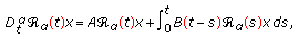 (2.5)
(2.5)
 is strongly continuous and
  for all
  and
and  .
. ,
,  , and
, and

for every  .
.
The existence of a resolvent operator for problem (2.3)-(2.4) was studied in [20]. In this paper, we have considered the following conditions.
-
(P1)
The operator
 is a closed linear operator with
  dense in
  . There is positive constants
  , such that
 (2.7)
(2.7)where
 ,
,  ,
,  for some
  , and
, and  for all
  .
. -
(P2)
For all
 ,
,  is a closed linear operator,
  , and
, and  is strongly measurable on
  for each
  . There exists
  (the notation
  stands for the set of all locally integrable functions from
  into
into  ) such that
  exists for
  and
and  for all
  and
and  . Moreover, the operator-valued function
  has an analytical extension (still denoted by
  ) to
) to  such that
  for all
  , and
, and  , as
, as  .
. -
(P3)
There exists a subspace
 dense in
  and positive constant
  , such that
  ,
,  ,
,  for every
  and all
  .
.
 is a closed linear operator with
  dense in
  . There is positive constants
  , such that
 ,
,  ,
,  for some
  , and
, and  for all
  .
. ,
,  is a closed linear operator,
  , and
, and  is strongly measurable on
  for each
  . There exists
  (the notation
  stands for the set of all locally integrable functions from
  into
into  ) such that
  exists for
  and
and  for all
  and
and  . Moreover, the operator-valued function
  has an analytical extension (still denoted by
  ) to
) to  such that
  for all
  , and
, and  , as
, as  .
. dense in
  and positive constant
  , such that
  ,
,  ,
,  for every
  and all
  .
.In the sequel, for  and
and  ,
,

for  ,
,  , are the paths

and  oriented counterclockwise. In addition,
  are the sets

We now define the operator family  by
by

The following result has been established in [20, Theorem 2.1].
Theorem 2.3.
Assume that conditions (P1)–(P3) are fulfilled, then there is a unique  -resolvent operator for problem (2.3)-(2.4).
In what follows, we always assume that the conditions (P1)–(P3) are verified.
We consider now the nonhomogeneous problem.
In the rest of this section, we discuss existence and regularity of solutions of


where  and
and  . In the sequel,
  is the operator function defined by (2.11). We begin by introducing the following concept of classical solution.
Definition 2.4.
A function  ,
,  is called a classical solution of (2.12)-(2.13) on
  if
if  ; the condition (2.13) holds and (2.12) is verified on
  .
.
Definition 2.5.
Let  , we define the family
  by
by

for each  .
.
The proof of the next result is in [20]. For reader's convenience, we will give the proof.
Lemma 2.6.
If the function  is exponentially bounded in
  , then
  is exponentially bounded in
  .
.
Proof.
If there are constants,  such that
  , we obtain

where  .
.
The next result follows from Lemma 2.6. We will omit the proof.
Lemma 2.7.
If the function  is exponentially bounded in
  , then
  is exponentially bounded in
  .
.
We now establish a variation of constants formula for the solutions of (2.12)-(2.13). The proof of the next result is in [20]. For reader's convenience, we will give the proof.
Theorem 2.8.
Let  . Assume that
  and
and  is a classical solution of (2.12)-(2.13) on
  , then

Proof.
The Cauchy problem (2.12)-(2.13) is equivalent to the Volterra equation

and the  -resolvent equation (2.6) is equivalent to

To prove (2.16), we notice that

Therefore,

We obtain

It is clear from the preceding definition that  is a solution of problem (2.3)-(2.4) on
  for
for  .
.
Definition 2.9.
Let  . A function
  is called a mild solution of (2.12)-(2.13) if

The proof of the next result is in [20]. For reader's convenience, we will give the proof.
Theorem 2.10.
Let  and
and  . If
. If  , then the mild solution of (2.12)-(2.13) is a classical solution.
Proof.
To begin with, we study the case in which  . Let
. Let  be the mild solution of (2.12)-(2.13) and assume that
  . It is easy to see that
  and
and

where  is given by
  . From [7, Lemma 3.12], we obtain that
  is a classical solution and satisfies

Moreover, from (2.24) and taking into account that  for all
  and
and  , we deduce the existence of constants
  ,
,  (which are independent from
  ) such that

Now, we assume that  . Let
. Let  be a sequence in
  such that
  in
in  . From [7, Lemma 3.12], we know that
  ,
,  , is a classical solution of (2.12)-(2.13) with
  in the place of
  . By using the estimate (2.25), we deduce the existence of functions
  , such that
  in
in  and
and  in
in  . These facts, jointly with our assumptions on
  , permit to conclude that
  in
in  . On the other hand,

we obtain

Now, by making  on
on

we conclude that  is a classical solution of (2.12)-(2.13). The proof is finished.
The proof of the next result is in [20]. For reader's convenience, we will give the proof.
Theorem 2.11.
Let  and
and  . If
. If  , then the mild solution of (2.12)-(2.13) is a classical solution.
Proof.
Let  , there is
  on
on  such that
  on
on  and
and  on
on  . Put
. Put  proceeding as in the proof of Theorem 2.10. It follows that
  is a classical solution of (2.12)-(2.13). Moreover, from [7, Lemma 3.13], we obtain

from which we deduce the existence of positive constants  (independent from
  ) such that

With similar arguments as in the proof of Theorem 2.10, we conclude that  is a classical solution of (2.12)-(2.13). We omit additional details. The proof is completed.
To establish our existence results, we need the following Lemma.
Lemma 2.12.
Let  . If
. If  is compact for some
  , then
  and
and  are compact for all
  .
.
Proof.
From the resolvent identity, it follows that  is compact for every
  . We have from [20, Lemma 2.2] that
  is a compact operator for
  ; therefore,
  is a compact operator for
  .
.
From [20, Lemma 2.5], we have,  is uniformly continuous for
  , for any
  fixed, we can select points
  , such that if
  , we obtain
  , for all
  and
and  .
.
Therefore, for all  , we have that

Noting now that

from (2.31), we find that

Thus,

where  is compact and
  , then we observe that
  as
as  . This permits us to conclude that
  is relatively compact in
  . This proves that
  is a compact operator for all
  .
.
For completeness, we include the following well-known result.
Theorem 2.13 (Leray-Schauder alternative, [21, Theorem  ]).
]).
Let  be a closed convex subset of a Banach space
  with
with  . Let
. Let  be a completely continuous map. Then,
  has a fixed point in
  or the set
  is unbounded.
3. Existence Results
In this section, we study the existence of mild solutions for system (1.1)-(1.2). Along this section,  is a positive constant such that
  and
and  for every
  . We adopt the notion of mild solutions for (1.1)-(1.2) from the one given in [20].
Definition 3.1.
A function  is called a mild solution of the neutral system (1.1)-(1.2) on
  if
if  ,
,  , and
, and

To prove our results, we always assume that  is continuous and that
  . If
. If  , we define
  as the extension of
  to
to  such that
  . We define
  such that
  where
where  is the extension of
  , such that
  for
for  .
.
In the sequel, we introduce the following conditions.
-
(H1)
The function
 verifies the following conditions:
-
(i)
the function
 is continuous for every
  , and for every
  , the function
  is strongly measurable,
 -
(ii)
there exist
 and a continuous nondecreasing function
  , such that
  , for all
  .
.
-
(i)
-
(H2)
For all
 ,
,  and
and  , the set
  is bounded in
  .
. -
(Hφ)
The function
 is well defined and continuous from the set
 (3.2)
(3.2)into
 , and there exists a continuous and bounded function
  , such that
  for every
  .
.
 verifies the following conditions:
 is continuous for every
  , and for every
  , the function
  is strongly measurable,
 and a continuous nondecreasing function
  , such that
  , for all
  .
. ,
,  and
and  , the set
  is bounded in
  .
. is well defined and continuous from the set
 , and there exists a continuous and bounded function
  , such that
  for every
  .
.Remark 3.2.
The condition  is frequently verified by continuous and bounded functions.
Remark 3.3.
In the rest of this section,  and
and  are the constants
  and
and  .
.
Lemma 3.4 (see [13, Lemma 2.1]).
Let  be continuous on
  and
and  . If
. If  holds, then

 , where
  .
.
Theorem 3.5.
Let conditions  ,
,  , and
, and  hold, and assume that
  . If
. If  , then there exists a mild solution of (1.1)-(1.2) on
  .
.
Proof.
Let  be the extension of
  to
to  such that
  on
on  . Consider the space
  endowed with the uniform convergence topology and define the operator
  by
by

for  . It is easy to see that
  . We prove that there exists
  such that
  . If this property is false, then for every
  there exist
  and
and  such that
  . Then, from Lemma 3.4, we find that

and hence,

which contradicts our assumption.
Let  be such that
  , in the sequel;
  and
and  are the numbers defined by
  and
and  . To prove that
  is a condensing operator, we introduce the decomposition
  , where

for  .
.
It is easy to see that  is continuous and a contraction on
  . Next, we prove that
  is completely continuous from
  into
into  .
.
Step 1.
Let  , and let
  be a positive real number such that
  . We can infer that

where  ,
,  is the convex hull of the set
  and
and  , since

which proves that  is relatively compact in
  .
.
Step 2.
The set  is equicontinuous on
  .
.
Let  and
and  such that
  for every
  with
with  . Under these conditions, for
  and
and  with
with  , we get

which shows that the set of functions  is right equicontinuity at
  . A similar procedure permits us to prove the right equicontinuity at zero and the left equicontinuity at
  . Thus,
  is equicontinuous. By using a similar procedure to proof of the [13, Theorem 2.3], we prove that that
  is continuous on
  , which completes the proof
  is completely continuous.
The existence of a mild solution for (1.1)-(1.2) is now a consequence of [22, Theorem  ]. This completes the proof.
Theorem 3.6.
Let conditions  ,
,  ,
,  hold,
hold,  for every
  , and assume that
  . If
. If

where  , then there exists a mild solution of (1.1)-(1.2) on
  .
.
Proof.
Let  be the operator defined by (3.4). In the sequel we use Theorem 2.13. If
  ,
,  , then from Lemma 3.4, we have that

since  for every
  . If
. If  , we obtain that

Denoting by  the right-hand side of the last inequality, we obtain that

and hence

This inequality and (3.11) permit us to conclude that the set of functions  is bounded, which in turn shows that
  is bounded.
By using a similar procedure allows to proof Theorem 3.5, we obtain that  is completely continuous. By Theorem 2.13, the proof is ended.
4. Example
To finish this section, we apply our results to study an integrodifferential equation which arises in the theory of heat equation. Consider the system

In this system,  ,
,  ,
,  are positive numbers and
  . To represent this system in the abstract form (1.1)-(1.2), we choose the spaces
  and
and  , see Example 2.1 for details. In the sequel,
  is the operator given by
  with domain
  . It is well known that
  is the infinitesimal generator of an analytic semigroup
  on
on  . Hence,
  is sectorial of type and (P1) is satisfied. We also consider the operator
  ,
,  ,
,  for
for  . Moreover, it is easy to see that conditions (P2)-(P3) in Section 2 are satisfied with
  and
and  , where
  is the space of infinitely differentiable functions that vanish at
  and
and  .
.
We next consider the problem of the existence of mild solutions for the system (4.1). To this end, we introduce the following functions:

Under the above conditions, we can represent the system (4.1) in the abstract form (2.12)-(2.13). The following result is a direct consequence of Theorem 3.5.
Proposition 4.1.
Let  be such that condition
  holds, the functions
  are bounded, and assume that the above conditions are fulfilled, then there exists a mild solution of (4.1) on
  .
.
References
Bartha M: Periodic solutions for differential equations with state-dependent delay and positive feedback. Nonlinear Analysis: Theory, Methods & Applications 2003,53(6):839-857. 10.1016/S0362-546X(03)00039-7
Cao Y, Fan J, Gard TC: The effects of state-dependent time delay on a stage-structured population growth model. Nonlinear Analysis: Theory, Methods & Applications 1992,19(2):95-105. 10.1016/0362-546X(92)90113-S
Domoshnitsky A, Drakhlin M, Litsyn E: On equations with delay depending on solution. Nonlinear Analysis: Theory, Methods & Applications 2002,49(5):689-701. 10.1016/S0362-546X(01)00132-8
Chen F, Sun D, Shi J: Periodicity in a food-limited population model with toxicants and state dependent delays. Journal of Mathematical Analysis and Applications 2003,288(1):136-146. 10.1016/S0022-247X(03)00586-9
Hartung F: Linearized stability in periodic functional differential equations with state-dependent delays. Journal of Computational and Applied Mathematics 2005,174(2):201-211. 10.1016/j.cam.2004.04.006
Hartung F: Parameter estimation by quasilinearization in functional differential equations with state-dependent delays: a numerical study. Nonlinear Analysis: Theory, Methods & Applications 2001,47(7):4557-4566. 10.1016/S0362-546X(01)00569-7
Hartung F, Herdman TL, Turi J: Parameter identification in classes of neutral differential equations with state-dependent delays. Nonlinear Analysis: Theory, Methods & Applications 2000,39(3):305-325. 10.1016/S0362-546X(98)00169-2
Kuang Y, Smith HL: Slowly oscillating periodic solutions of autonomous state-dependent delay equations. Nonlinear Analysis: Theory, Methods & Applications 1992,19(9):855-872. 10.1016/0362-546X(92)90055-J
Torrejón R: Positive almost periodic solutions of a state-dependent delay nonlinear integral equation. Nonlinear Analysis: Theory, Methods & Applications 1993,20(12):1383-1416. 10.1016/0362-546X(93)90167-Q
Li Y: Periodic solutions for delay Lotka-Volterra competition systems. Journal of Mathematical Analysis and Applications 2000,246(1):230-244. 10.1006/jmaa.2000.6784
dos Santos JPC: On state-dependent delay partial neutral functional integro-differential equations. Applied Mathematics and Computation 2010,216(5):1637-1644. 10.1016/j.amc.2010.03.019
dos Santos JPC: Existence results for a partial neutral integro-differential equation with state-dependent delay. Electronic Journal of Qualitative Theory of Differential Equations 2010,2010(29):1-12.
Hernández E, Prokopczyk A, Ladeira L: A note on partial functional differential equations with state-dependent delay. Nonlinear Analysis: Real World Applications 2006,7(4):510-519. 10.1016/j.nonrwa.2005.03.014
Hernández M E, McKibben MA: On state-dependent delay partial neutral functional-differential equations. Applied Mathematics and Computation 2007,186(1):294-301. 10.1016/j.amc.2006.07.103
Hernández Morales E, McKibben MA, Henríquez HR: Existence results for partial neutral functional differential equations with state-dependent delay. Mathematical and Computer Modelling 2009,49(5-6):1260-1267. 10.1016/j.mcm.2008.07.011
Maraaba T, Baleanu D, Jarad F: Existence and uniqueness theorem for a class of delay differential equations with left and right Caputo fractional derivatives. Journal of Mathematical Physics 2008,49(8):-11.
Maraaba T, Jarad F, Baleanu D: On the existence and the uniqueness theorem for fractional differential equations with bounded delay within Caputo derivatives. Science in China Series A 2008,51(10):1775-1786. 10.1007/s11425-008-0068-1
Agarwal R, de Andrade B, Siracusa G: On fractional integro-differential equations with state-dependent delay. to appear in Computers & Mathematics with Applications
Hino Y, Murakami S, Naito T: Functional-Differential Equations with Infinite Delay, Lecture Notes in Mathematics. Volume 1473. Springer, Berlin, Germany; 1991:x+317.
Agarwal R, dos Santos JPC, Cuevas C: Analytic resolvent operator and existence results for fractional integro-differential equations. submitted
Granas A, Dugundji J: Fixed Point Theory, Springer Monographs in Mathematics. Springer, New York, NY, USA; 2003:xvi+690.
Martin RH Jr.: Nonlinear Operators and Differential Equations in Banach Spaces. Robert E. Krieger Publishing, Melbourne, Fla, USA; 1987:xiv+440.
Acknowledgments
The final version of this paper was finished while the third author was visiting the Universidade Federal de Pernambuco (Recife, Brasil) during Desember 2010-January 2011. The third author would like to thank the Functional Equations Group for their kind invitation and hospitality. The authors are grateful to the referees for pointing out omissions and misprints, and demanding vigorously details and clarifications. J. P. C. dos Santos is partially supported by FAPEMIG/Brazil under Grant no. CEX-APQ-00476-09. C. Cuevas is partially supported by CNPQ/Brazil under Grant no. 300365/2008-0. B. de Andrade is partially supported by CNPQ/Brazil under Grant no. 100994/2011-3.
Author information
Authors and Affiliations
Corresponding author
Rights and permissions
Open Access This article is distributed under the terms of the Creative Commons Attribution 2.0 International License ( https://creativecommons.org/licenses/by/2.0 ), which permits unrestricted use, distribution, and reproduction in any medium, provided the original work is properly cited.
About this article
Cite this article
dos Santos, J.P.C., Cuevas, C. & de Andrade, B. Existence Results for a Fractional Equation with State-Dependent Delay. Adv Differ Equ 2011, 642013 (2011). https://doi.org/10.1155/2011/642013
Received:
Revised:
Accepted:
Published:
DOI: https://doi.org/10.1155/2011/642013