Difference-differential operators for basic adaptive discretizations and their central function systems

Abstract

The concept of inherited orthogonality is motivated and an optimality statement for it is derived. Basic adaptive discretizations are introduced. Various properties of difference operators which are directly related to basic adaptive discretizations are looked at. A Lie-algebraic concept for obtaining basic adaptive discretizations is explored. Some of the underlying moment problems of basic difference equations are investigated in greater detail.

1 Introduction and motivation

The wide area of ordinary differential equations and various types of ordinary difference equations is always closely connected to special function systems. Essential contributions have been added through the last century linking concepts of functional analysis to the world of differential equations and difference equations.

Difference equations are usually understood in the sense of equidistant differences. However, new and attractive discretizations, like adaptive discretizations come in. The intention of this article is to address specific problems which are related to so-called basic adaptive discretizations: Starting from conventional difference and differential equations, we move on to basic difference equations.

In Section 2, we motivate creating new types of orthogonal polynomials from a given orthogonal polynomial system. Ingredients like tripolynomial function classes, node integrals, and some properties of the classical Hermite polynomials are revised.

Section 3 addresses the concept of inherited orthogonality - transferring orthogonality from one generation of orthogonal polynomials to the next one. It contains an optimality statement for computing properties which links two different generations of functions.

In Section 4, the concept of basic adaptive discretization is presented and the underlying Lie-algebra structure of discrete Heisenberg algebras is given.

Having worked on special functions related to differential equations, we explore in some more detail the world of discrete functions being related to basic adaptive discretizations in Section 5. There, we look in greater detail at solutions of underlying moment problems.

Let us briefly mention some preceding work:

Reference [1] was an important starting point to initiate results of this present article. Reference [2] refers to the ladder operator formalism in discrete Schrödinger theory. A wide survey of results stemming from discrete Schrödinger theory is provided through [3]. In discrete Schrödinger theory, basic special functions like q-hypergeometric functions resp. related orthogonal polynomials play a prominent role when solving the underlying Schrödinger difference equations. Central properties of these functions are outlined for instance in [4, 5]. The application of basic difference equations to formulating discrete diffusion processes has been addressed in [6, 7].

2 Towards new generations of orthogonality

The main philosophy of this section shall be as follows:

Given a sequence of orthogonal polynomials, let us take one particular of its family members and call it father polynomial. We are interested in the calculation of the node integrals for this father polynomial.

Calculating the moments of the respective positivity parts of the father polynomial, one obtains all information on further systems of orthogonal polynomials which are based on the father polynomial.

We call them daughter polynomials. They oscillate between the nodes of the father polynomial. The higher the index of a daughter polynomial in the new class of orthogonal polynomials gets, the wilder is the daughter polynomial ‘dancing’: All its nodes are located between the nodes of the father polynomial, i.e., the higher the oscillations of a particular daughter polynomial get, the more nodes of the daughter polynomial can be found between the nodes of the original father polynomial.

In order to proceed into this direction, let us put some ingredients together.

Definition 2.1 Let $F:=\{F_0,F_1,F_2,F_3,\dots \}$ be an orthogonal polynomial system where for $F_j$ the degree is given by j. By $\mathcal{K}(F)$, we understand the set of all function systems which are collinear with the elements of F. Note that 0 shall be excluded from this set. We call $\mathcal{K}(F)$ the tripolynomial function class of the function system F.

Let $p:\mathbb{R}\to \mathbb{R}$ be a polynomial of degree k with at least two zeros. The zeros of the polynomials shall be denoted by $z_1,\dots ,z_j$ where $j\le k-2$, they are also called nodes.

We call two nodes of the polynomial adjacent if there exists no further node of p between these two nodes.

The nodes $z_1,\dots ,z_j$ shall be arranged such that $z_1$ and $z_2$ are adjacent. Without loss of generality, such an arrangement is always possible in view of the given conditions.

For $n\in {\mathbb{N}}_0$, we call the integrals

$${\int }_{z_1}^{z_2}{x}^{n}p(x)dx$$

(1)

node integrals of the polynomial p.

To see how the orthogonality and its oscillations are inherited from one generation to the next, we will combine the stated ingredients to formulate the corresponding analytic statements which will appear in Theorem 3.2. This theorem will contain an existence and optimality statement for predicting some properties of daughter polynomials: In the case of the Hermite polynomials, this can be done in an optimal way, i.e., there one can find an optimal way for calculating the node integrals from the original father polynomials. Let us briefly summarize some of their classical properties which will play an important role when deriving new results in the next section:

Lemma 2.2 (Properties of the classical Hermite polynomials)

Starting from the function

$$G_0:\mathbb{R}\to \mathbb{R},x\mapsto G_0(x):=e^{-x^2},$$

(2)

we define for $n\in {\mathbb{N}}_0$ and $x\in \mathbb{R}$ the functions $G_n$ successively as follows:

$$G_{n+1}(x)=-G_n^{\prime }(x).$$

(3)

For $n\in {\mathbb{N}}_0$, the nth Hermite polynomial is then introduced as

$$H_n:\mathbb{R}\to \mathbb{R},x\mapsto H_n(x):=e^{x^2}{G}_n(x).$$

(4)

The Hermite polynomials satisfy for $x\in \mathbb{R}$ and $n\in {\mathbb{N}}_0$ the equations

(5)

(6)

Let $p,q\in M$ be the vector space of all real-valued polynomials over $\mathbb{R}$. We obtain an orthogonality statement between p and q with respect to the Euclidean scalar product

$$(p,q):={\int }_{-\mathrm{\infty }}^{\mathrm{\infty }}p(t)q(t)e^{-t^2}dt,$$

(7)

namely: The Hermite polynomials are pairwise orthogonal with respect to (7). For two different $m,n\in {\mathbb{N}}_0$, we receive

$${\int }_{-\mathrm{\infty }}^{\mathrm{\infty }}{H}_m(t)H_n(t)e^{-t^2}dt=0.$$

(8)

Moreover, for all $m\in {\mathbb{N}}_0$, the following strict inequality holds:

$$0<{\int }_{-\mathrm{\infty }}^{\mathrm{\infty }}{H}_m(t)H_m(t)e^{-t^2}dt<\mathrm{\infty }.$$

(9)

3 The oscillations of inherited orthogonality

In the sequel, our aim is to derive some general statements on node integrals of orthogonal polynomial systems, i.e., we are interested in integrals of type

$${\int }_{z_1}^{z_2}{x}^n{P}_j(x)dx,$$

(10)

where $P_j$ is a fixed function of an orthogonal polynomial system P, $z_1$, and $z_2$ being adjacent nodes of $P_j$. For a fixed value $j\in {\mathbb{N}}_0$, we start from the defining equation

$$a_{j+2}{P}_{j+2}(x)-x{b}_{j+1}{P}_{j+1}(x)+c_j{P}_j(x)=d_j{P}_{j+1}(x).$$

(11)

Rewriting identity (11), we first obtain

$$x{b}_{j+1}{P}_{j+1}(x)=a_{j+2}{P}_{j+2}(x)+c_j{P}_j(x)-d_j{P}_{j+1}(x).$$

(12)

Dividing by the b-coefficients, we receive

$$x{P}_{j+1}(x)=\frac{a_{j+2}}{b_{j+1}}{P}_{j+2}(x)+\frac{c_j}{b_{j+1}}{P}_j(x)-\frac{d_j}{b_{j+1}}{P}_{j+1}(x).$$

(13)

Applying now the procedure (13) for the calculation of $x^n{P}_{j+1}(x)$ in a successive way, we get

$$x^n{P}_{j+1}(x)=c_{n+j+1}^{(n,j)}{P}_{n+j+1}(x)+c_{n+j}^{(n,j)}{P}_{n+j}(x)+\cdots +c_0^{(n,j)}{P}_0(x).$$

(14)

Note that the coefficients

$$c_{n+j+1}^{(n,j)},c_{n+j}^{(n,j)},\dots ,c_0^{(n,j)}$$

(15)

are uniquely fixed through the calculation procedure (13). In terms of the sigma notation, we can reformulate Eq. (14) in the following short-hand way:

$$x^n{P}_{j+1}(x)=\sum _{k=0}^{n+j+1}{c}_k^{(n,j)}{P}_k(x).$$

(16)

The bracket notation $(n,j)$ at the different coefficients $c_k^{(n,j)}$ indicates that the coefficients depend indeed on a fixed chosen number $j\in {\mathbb{N}}_0$ and from $n\in {\mathbb{N}}_0$ in $x^n$. Due to their importance, these coefficients deserve a special name which will be given by the following.

Definition 3.1 (Structure coefficients)

The coefficients $c_k^{(n,j)}$ stemming from the procedure specified in (14) through (16) are called structure coefficients of the polynomial $P_{j+1}$.

The structure coefficients depend on the fixed value of the power $n\in {\mathbb{N}}_0$ on the left-hand side of (16) as well as on the fixed value of the power $j\in {\mathbb{N}}_0$ of the polynomial index of $P_{j+1}$ - moreover they depend additionally on the counting index k. The number k starts from the value 0 and runs from 1 through $n+j+1$.

Calculating the node integrals on the left-hand side of (16) yields

$${\int }_{z_1}^{z_2}{x}^n{P}_{j+1}(x)dx={\int }_{z_1}^{z_2}(\sum _{k=0}^{n+j+1}{c}_k^{(n,j)}{P}_k(x))dx=\sum _{k=0}^{n+j+1}{c}_k^{(n,j)}{\int }_{z_1}^{z_2}{P}_k(x)dx.$$

(17)

This identity is the starting point for a fascinating analytic path. One may ask the question of how to find an optimal algorithm linking the following three sequences of data:

• the node integrals which can be obtained by direct integration:

  $${\mu }_{n,j}:={\int }_{z_1}^{z_2}{x}^n{P}_j(x)dx$$

  (18)

• the values of all polynomials $P_m$ at two adjacent nodes of a special $P_j$:

  $$P_m(z_1),P_m(z_2)$$

  (19)

• the structure coefficients $c_k^{(n,j)}$.

To get this procedure started, we assume j, k, m and n as suitably chosen indices.

This task can be approached on a more general level in the following theorem, leading even to an unexpected optimality statement.

Theorem 3.2 (New generations of orthogonality)

Let $P_j$ be the jth polynomial of an orthogonal polynomial system. Moreover, let $z_1$ and $z_2$ be two adjacent nodes of this polynomial. Without loss of generality, we assume that $P_j$ between $z_1$ and $z_2$ is nonnegative. Under these assertions, the following statements hold:

• (1) The evaluation of all elements $P_m$ ($m\in {\mathbb{N}}_0$) of the tripolynomial function system at two adjacent nodes $z_1$ and $z_2$ of the particular polynomial $P_j$ yields complete information on a sequence of new polynomials $T_n$ ($n\in {\mathbb{N}}_0$). These polynomials are defined for $z_1\le x\le z_2$ and have for all pairwise different $m,n\in {\mathbb{N}}_0$ the following properties:

  

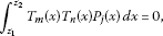  (20)
  

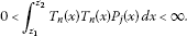  (21)

• (2) Each of the $T_n$ - without $T_0$ - changes its sign between $z_1$ and $z_2$, i.e., is oscillatory between the integration boundaries $z_1$ and $z_2$.

• (3) In the case of an orthogonal polynomial system, each of the polynomials $P_j$ contains information on a complete set of new orthogonal polynomials: Starting from $P_j$, the orthogonality is inherited to the $T_n$ ($n\in {\mathbb{N}}_0$).

• (4) In this context, we have the following Existence and Optimality Statement:

Using the data $P_m(z_1)$, $P_m(z_2)$ ($m\in {\mathbb{N}}_0$), one obtains in the case of the Hermite polynomials an optimal algorithm while calculating the node integrals

$${\int }_{z_1}^{z_2}{x}^n{P}_j(x)dx,n\in {\mathbb{N}}_0.$$

(22)

• (5) Moreover, the following Uniqueness Statement holds:

The Hermite polynomials are the only tripolynomial function class of analysis which shows an optimality property when calculating (22) using the data $P_m(z_1)$, $P_m(z_2)$ while m is ranging in ${\mathbb{N}}_0$.

Proof (1) For a fixed value of $j\in {\mathbb{N}}_0$ the polynomial $P_j$ does not change its sign between two different adjacent nodes. The existence of nodes is guaranteed through the orthogonality properties of the whole polynomial sequence ${(P_k)}_{k\in n\in {\mathbb{N}}_0}$.

Suppose now that $z_1$ and $z_2$ are two adjacent nodes of $P_j$ where we assume without of loss of generality that the father polynomial $P_j$ is nonnegative between $z_1$ and $z_2$. In particular, the father polynomial is positive in the open interval $(z_1,z_2)$ and vanishing in $z_1$ and $z_2$. According to the properties of continuous functions on compact intervals, all node integrals (22) exist for $P_j$ and are positive. By means of the outlined standard procedures, we can construct from these node integrals a new sequence of orthogonal polynomials, the daughter polynomials ${(T_n)}_{n\in n\in {\mathbb{N}}_0}$. This reflects precisely the statements (20) and (21).

• (2) According to the orthogonality relations, (20) follows that the daughter polynomials must change their signs in the open interval $(z_1,z_2)$. And according to general results on orthogonal polynomials ${(T_n)}_{n\in n\in {\mathbb{N}}_0}$, it follows moreover that the higher the index n gets the more oscillatory $T_n$ behaves.

• (3) Starting now from a tripolynomial function system with given orthogonality measure, each of its pairwise orthogonal polynomials $P_j$ inherits through the procedure outlined in (1) and (2) its orthogonality to the sequence ${(T_n)}_{n\in n\in {\mathbb{N}}_0}$.

• (4) In the case of the classical Hermite polynomials, one sees that thanks to their differential equation (5) and making use of the expansion (17), there is an optimal effort for calculating the node integrals of a particular Hermite polynomial from the evaluation of all other Hermite polynomials at the two fixed nodes of the particular polynomial.

Polynomials not having a similar differential equation (5) need a longer sequence of computational steps to evaluate the node integrals of a particular polynomial from the values of all polynomials at the two nodes of the considered particular polynomial.

• (5) The concept of optimality is closely tied to the differential equation (5): The fact that the derivative of a polynomial in a tripolynomial system is a multiple value of its predecessor is characteristic for the tripolynomial function class of Hermite polynomials - and only for them - as direct calculation shows. This yields the uniqueness statement. □

4 Adaptive discretization and basic Heisenberg algebras

We have so far worked in this article on difference equations, namely orthogonal polynomial systems connecting members of a function family. They are solutions to a particular differential equation.

This is, for instance, one of the standard scenarios in conventional quantum mechanics where the Hermite functions, the Laguerre functions, and the Legendre functions play particular roles in different physical situations. The main spirit among these functions is always a continuous one. We now move to describing discretized function systems and to discovering the algebraic structures behind one special type of fancy discretization: the basic adaptive discretization.

Definition 4.1 (Basic adaptive discretization)

Let Ω be a nonvanishing subset of the real axis having a characteristic function ${\chi }^{\mathrm{\Omega }}$ with properties

$${\chi }^{\mathrm{\Omega }}(qx)={\chi }^{\mathrm{\Omega }}\left(q^{-1}x\right)={\chi }^{\mathrm{\Omega }}(x),x\in \mathbb{R},$$

(23)

where Ω may be the real axis by itself. The number $0<q<1$ is chosen always as a fixed number. For a real-valued function $f:\mathrm{\Omega }\to \mathbb{R}$, we define the first basic discrete grid operation by

$$(Xf)(x):=xf(x)$$

(24)

and the second basic discrete grid operation resp. its inverse through

$$(Rf)(x):=f(qx),(Lf)(x):=f\left(q^{-1}x\right).$$

(25)

We introduce as a metric structure on suitable subsets of the linear function space $F(\mathrm{\Omega },\mathbb{C})$ of all complex-valued functions on Ω the Euclidean scalar product

$${(f,g)}_{\mathrm{\Omega }}:={\int }_{-\mathrm{\infty }}^{\mathrm{\infty }}f(x)\overline{g(x)}{d}_{{\chi }^{\mathrm{\Omega }}}^x$$

(26)

with corresponding Lebesgue-integration measure and obtain hence the canonical norm through

$${\parallel f\parallel }_{\mathrm{\Omega }}:=\sqrt{{(f,f)}_{\mathrm{\Omega }}}.$$

(27)

From these structures, it becomes apparent what the corresponding Lebesgue spaces ${\mathcal{L}}^p(\mathrm{\Omega })$ are.

Remark 4.2 Let us concentrate on two different realizations of the Lebesgue integration measure $d_{{\chi }^{\mathrm{\Omega }}}^x$, namely in the first case on a purely discrete measure and in the second case on a measure stemming from a set Ω with properties (23) having itself a positive Lebesgue measure, i.e., $\mu (\mathrm{\Omega })>0$. This second case corresponds to piecewise-continuous realizations of the integration measure; we will refer to them also in the fifth chapter by the name basic layers.

Hence, the two different integration measures are related to the respective scalar products of the form

$${(f,g)}_{\mathrm{\Omega }}=\sum _{k=-\mathrm{\infty }}^{\mathrm{\infty }}r{q}^{k}f\left(r{q}^k\right)\overline{g\left(r{q}^k\right)}+\sum _{k=-\mathrm{\infty }}^{\mathrm{\infty }}s{q}^{k}f{(-s{q}^k)}^n\overline{g(-s{q}^k)}$$

(28)

in the purely discrete scenario where r, s are two fixed positive numbers, and

$${(f,g)}_{\mathrm{\Omega }}:={\int }_{-\mathrm{\infty }}^{\mathrm{\infty }}f(x)\overline{g(x)}{\chi }^{\mathrm{\Omega }}(x)dx$$

(29)

in the piecewise-continuous basic layer case with $\mu (\mathrm{\Omega })>0$.

Already for the discrete case, and there in the situation of real-valued f, g with compact support, it can be shown by direct inspection that

$${(Xf,g)}_{\mathrm{\Omega }}={(f,Xg)}_{\mathrm{\Omega }},{(Rf,g)}_{\mathrm{\Omega }}=q^{-1}{(f,Lg)}_{\mathrm{\Omega }}.$$

(30)

To illustrate this fact in the case of R for instance, let us without loss of generality restrict to those real-valued functions f, g with compact support, vanishing on the s-part of the lattice Ω such that

$${(Rf,g)}_{\mathrm{\Omega }}=\sum _{k=-\mathrm{\infty }}^{\mathrm{\infty }}r{q}^k(Rf)\left(r{q}^k\right)g\left(r{q}^k\right)=\sum _{k=-\mathrm{\infty }}^{\mathrm{\infty }}r{q}^{k}f\left(r{q}^{k+1}\right)g\left(r{q}^k\right)\overline{g(-s{q}^k)}.$$

(31)

We find furthermore that the expression on the very right-hand side of (31) equals to

$$\sum _{k=-\mathrm{\infty }}^{\mathrm{\infty }}r{q}^{k-1}f\left(r{q}^k\right)g\left(r{q}^{k-1}\right)=q^{-1}\sum _{k=-\mathrm{\infty }}^{\mathrm{\infty }}r{q}^{k}f\left(r{q}^k\right)(Lg)\left(r{q}^k\right)\overline{g(-s{q}^k)}$$

(32)

which confirms the statement - the more general situation of the full lattice being similar. This finally allows us to introduce X, R, L as linear operators acting on all complex-valued functions which have compact support on the grid

$$\mathrm{\Omega }=\{r{q}^k\mid k\in \mathbb{Z}\}\cup \{-s{q}^k\mid k\in \mathbb{Z}\}.$$

(33)

In this sense, there exists a formal adjointness star operation such that

$$X^{\ast }=X,R^{\ast }=q^{-1}L=q^{-1}{R}^{-1},L^{\ast }=qR.$$

(34)

In this sense, we speak of X as a formally symmetric operator.

Note that one can easily find the same adjointness relations (34) in the case of the integration measure (29) using similarly suitable domains for the three operators X, R, L.

Lemma 4.3 (Properties of some basic discretizers)

Let for $m,n\in \mathbb{Z}$ the basic discretizers be the linear operators, stemming from X, R, L with compact domains in ${\mathcal{L}}^2(\mathrm{\Omega })$ related to the scalar product (28):

(35)

(36)

(37)

We then have in all cases with respect to (28) the adjointness properties

$${\left(Q_n^m\right)}^{\ast }=Q_n^m,{\left(D_n^m\right)}^{\ast }=-D_n^m,{\left(P_n^m\right)}^{\ast }=P_n^m.$$

(38)

Proof Let us restrict for simplicity on the case of $Q_n^m$, the proof for the D-objects resp. P-objects being performed similar. Since the operators $X,R,L=R^{-1}$ are defined on compact domains of the ${\mathcal{L}}^2(\mathrm{\Omega })$ under consideration, we obtain

$${\left(Q_n^m\right)}^{\ast }={(X^m{R}^n+q^{-n}{R}^{-n}{X}^m)}^{\ast }={\left(R^n\right)}^{\ast }{\left(X^m\right)}^{\ast }+q^{-n}{\left(X^m\right)}^{\ast }{\left(R^{-n}\right)}^{\ast }$$

(39)

$$={\left(R^{\ast }\right)}^n{\left(X^{\ast }\right)}^m+q^{-n}{\left(X^{\ast }\right)}^m{\left(R^{\ast }\right)}^{-n}=q^{-n}{R}^{-n}{X}^m+q^{-n}{X}^m{q}^n{R}^n$$

(40)

$$=q^{-n}{R}^{-n}{X}^m+X^m{R}^n=Q_n^m.$$

(41)

Deriving these properties, we have in detail made use of standard operator theoretical results on compactly defined linear operators with respect to star operations. □

Remark 4.4 In the sequel - throughout the end of this section - we will also make use of the properties

$$RX=qXR,LX=q^{-1}XL$$

(42)

which hold on the domains for X, R, L and their products. Moreover, we define the anticommutator bracket and the commutator bracket between the objects going to appear in Theorem 4.5 via

$$\{A,B\}=AB+BA,[A,B]=AB-BA.$$

(43)

Building all these structures from Lemma 4.3 and Remark 4.4 together, one obtains by elementary but tedious calculations the full structure of the underlying basic Heisenberg algebra which is going to reveal its beauty in the following Theorem 4.5. Note, in particular, that the Jacobi identity which is an essential ingredient to verifying the Lie-algebra structure can be addressed straight. This happens thanks to the associative behavior of the operators X, R, L in basic adaptive discretizations.

Theorem 4.5 (Lie-algebraic structures of basic Heisenberg relations)

Let in the sequel $j,k,m,n\in \mathbb{Z}$ be arbitrary. We then have the following anticommutator relations between the formally symmetric Q-objects and the formally antisymmetric D-objects:

(44)

(45)

(46)

The corresponding commutator relations look as follows:

(47)

(48)

(49)

Using the formally symmetric P-objects, the anticommutator relations become

(50)

(51)

(52)

and we finally end up with the Lie algebra between the formally symmetric Q-discretizers and the formally symmetric P-discretizers as follows:

(53)

(54)

(55)

5 Moment problems and basic difference equations

Having looked at the basic discretization process by itself in the last section, the starting point for this section are now basic difference equations as concrete basic objects, namely

$$\sum _{j=0}^m{a}_j{x}^{2j}f(qx)=\sum _{j=0}^{m+1}{b}_j{x}^{2j}f(x),m\in {\mathbb{N}}_0$$

(56)

with suitable nonnegative $a_j$-coefficients and $b_j$-coefficients. We want to investigate some specific moment problems related to it.

To do so, let us first have a look at the structures which will come in. Like in the previous section, we will always assume $0<q<1$.

Definition 5.1 (Continuous structures in use)

Throughout the sequel, we will make use of the multiplication operator and shift-operator, their actions being given by

$$(X\phi )(x):=x\phi (x),(R\phi )(x):=\phi (qx)$$

(57)

on suitable definition ranges. We define the linear functional $K_0:{\mathcal{L}}^1(\mathbb{R})\to \mathbb{R}$ by

$$K_0(f):={\int }_{-\mathrm{\infty }}^{\mathrm{\infty }}f(x)dx$$

(58)

and successively for arbitrary $n\in \mathbb{N}$ the linear functionals $K_n$ on their maximal domains $D(K_n)\subseteq {\mathcal{L}}^1(\mathbb{R})$ via

$$K_n(f):={\int }_{-\mathrm{\infty }}^{\mathrm{\infty }}{x}^{n}f(x)dx$$

(59)

provided the integral in (59) exists in all cases.

We are now going to formulate a technical result concerning solutions to (56) which will be a helpful tool to the investigations in the sequel.

Lemma 5.2 (Extension property for continuous solutions)

Let us consider for a fixed number $m\in \mathbb{N}$ the basic difference equation

$$\sum _{j=0}^m{a}_j{X}^{2j}Rf=\sum _{j=0}^{m+1}{b}_j{X}^{2j}f,$$

(60)

where we assume that $a_0,a_1,\dots ,a_m$, $b_0,b_1,\dots ,b_{m+1}$ are nonnegative numbers. We require additionally $a_m{b}_{m+1}>0$ and $a_0{b}_0>0$. Let moreover for two arbitrary but fixed $j,k\in \mathbb{Z}$ the sets

$$J_j^{+}:=(q^{j+1},q^j),J_k^{-}:=(-q^k,-q^{k+1})$$

(61)

be given and let the function $u:J_j^{+}\cup \{q^j\}\cup \{q^{j+1}\}\to {\mathbb{R}}_0^{+}$, $x\mapsto u(x)$ as well as the function $v:J_k^{-}\cup \{-q^k\}\cup \{-q^{k+1}\}\to {\mathbb{R}}_0^{+}$, $x\mapsto v(x)$ be continuous and in particular in agreement with (56) resp. (60) where at most u or v exclusively is allowed to be the zero function in the sense of the Lebesgue integral.

Then u together with v can be extended via (60) to one single positive solution $f\in {\mathcal{L}}^1(\mathbb{R})$ which is in any case continuous on $\mathbb{R}\setminus \{0\}$. The action of all $K_n$ on both hand sides of (60) yields

$$K_n\left(\sum _{j=0}^m{a}_j{X}^{2j}Rf\right)=K_n\left(\sum _{j=0}^{m+1}{b}_j{X}^{2j}f\right)$$

(62)

transforming into the moment equation

$$\sum _{j=0}^m{a}_j{q}^{-2j-n-1}{K}_{n+j}(f)=\sum _{j=0}^{m+1}{b}_j{K}_{n+j}(f).$$

(63)

Proof Rewriting (60) in the form of (56), one recognizes that the extension process from u together with v to f is standard. By conventional analytic arguments, the existence of all moments of f can be concluded. Hence, in particular, we have $f\in {\mathcal{L}}^1(\mathbb{R})$, where $f(0)$ has to be specified since it does not come out of the extension process.

The choice of $f(0)$ may in particular be arbitrary since this does not violate the property $f\in {\mathcal{L}}^1(\mathbb{R})$. By analytic standard arguments of integration, one may conclude that (62) and (63) are for all $n\in {\mathbb{N}}_0$ well defined. These observations practically conclude all steps while verifying the technical Lemma 5.2. □

Remark 5.3 We would like to point out that Lemma 5.2 already provides a plenty of possible solutions to (60). Let, for instance, ${(f_k)}_{k\in {\mathbb{N}}_0}$ be a sequence of functions in the sense of Lemma 5.2 and ${({\gamma }_k)}_{k\in {\mathbb{N}}_0}$ be a sequence of nonnegative numbers where only finitely many of them are different from zero. The linear combination

$$g:=\sum _{k=0}^{\mathrm{\infty }}{\gamma }_k{f}_k$$

(64)

is then again a solution to (60) in the sense of Lemma 5.2: The function g is in any case continuous in $\mathbb{R}\setminus \{0\}$ and is in the maximal domain of K. Hence, the application of all the integration functionals $K_n$ ($n\in {\mathbb{N}}_0$) on the equation

$$\sum _{j=0}^m{a}_j{X}^{2j}Rg=\sum _{j=0}^{m+1}{b}_j{X}^{2j}g$$

(65)

leads to the moment equation

$$\sum _{j=0}^m{a}_j{q}^{-2j-m-1}{K}_{n+j}(g)=\sum _{j=0}^{m+1}{b}_j{K}_{n+j}(g),m\in {\mathbb{N}}_0.$$

(66)

Having shed some light on continuous solutions of the basic difference equation (60), let us now look at restrictions of the continuous solutions to special intervals. To do so, let us confine to subsets of the real axis for which the characteristic function is invariant under the shift operator R from (57) respectively its inverse. We have

Theorem 5.4 (Existence of basic layer solutions)

Let f be a continuous positive solution of (60) on $\mathbb{R}\setminus \{0\}$. We look at a basic layer Ω which is a subset of the real axis with positive Lebesgue measure having a characteristic function ${\chi }^{\mathrm{\Omega }}$ with properties

$${\chi }^{\mathrm{\Omega }}(qx)={\chi }^{\mathrm{\Omega }}\left(q^{-1}x\right)={\chi }^{\mathrm{\Omega }}(x),x\in \mathbb{R}.$$

(67)

The application of all the integration functionals $K_n$ ($n\in {\mathbb{N}}_0$) on the equation

$${\chi }^{\mathrm{\Omega }}(X)\sum _{j=0}^m{a}_j{X}^{2j}Rf={\chi }^{\mathrm{\Omega }}(X)\sum _{j=0}^{m+1}{b}_j{X}^{2j}f$$

(68)

again leads to a moment equation of type (63) resp. (66),

$$\sum _{j=0}^m{a}_j{q}^{-2j-n-1}{K}_{n+j}(f_{\mathrm{\Omega }})=\sum _{j=0}^{m+1}{b}_j{K}_{n+j}(f_{\mathrm{\Omega }}),n\in {\mathbb{N}}_0,$$

(69)

where we have used the abbreviation

$$f_{\mathrm{\Omega }}:={\chi }^{\mathrm{\Omega }}(X)f={\chi }^{\mathrm{\Omega }}\circ f.$$

(70)

Proof Let us illustrate the scenario at the example

$$(a+b{x}^2)f(qx)=(c+d{x}^2+e{x}^4)f(x),x\in \mathbb{R}$$

(71)

where a, b, c, d, e fulfill the respective roles of the coefficients specified in the assertions of Lemma 5.2. We choose now Ω such that the conditions of Theorem 5.4 are fulfilled. Hence, we obtain

$${\chi }^{\mathrm{\Omega }}(x)(a+b{x}^2)f(qx)={\chi }^{\mathrm{\Omega }}(x)(c+d{x}^2+e{x}^4)f(x),x\in \mathbb{R}.$$

(72)

According to the properties (67), we can replace the expression ${\chi }^{\mathrm{\Omega }}(x)$ on the left-hand side of (72) by ${\chi }^{\mathrm{\Omega }}(qx)$:

$${\chi }^{\mathrm{\Omega }}(qx)(a+b{x}^2)f(qx)={\chi }^{\mathrm{\Omega }}(x)(c+d{x}^2+e{x}^4)f(x),x\in \mathbb{R}.$$

(73)

Integration of the last equality yields

$${\int }_{-\mathrm{\infty }}^{\mathrm{\infty }}{\chi }^{\mathrm{\Omega }}(qx)(a+b{x}^2)f(qx)dx={\int }_{-\mathrm{\infty }}^{\mathrm{\infty }}{\chi }^{\mathrm{\Omega }}(x)(c+d{x}^2+e{x}^4)f(x)dx.$$

(74)

Now we see that it is advantageous to use the symmetry property (67). We obtain by substitution

$$q^{-1}{\int }_{-\mathrm{\infty }}^{\mathrm{\infty }}{\chi }^{\mathrm{\Omega }}(x)(a+b{q}^{-2}{x}^2)f(x)dx={\int }_{-\mathrm{\infty }}^{\mathrm{\infty }}{\chi }^{\mathrm{\Omega }}(x)(c+d{x}^2+e{x}^4)f(x)dx.$$

(75)

This step can be generalized by the application of all moment generating functionals, yielding

$$q^{-n-1}(a{K}_n(f_{\mathrm{\Omega }})+b{q}^{-2}{K}_{n+2}(f_{\mathrm{\Omega }}))=c{K}_n(f_{\mathrm{\Omega }})+d{K}_{n+2}(f_{\mathrm{\Omega }})+e{K}_{n+4}(f_{\mathrm{\Omega }}).$$

(76)

Here, we see that the specific structure of Ω does not influence the moment equality - what all moment equalities of type (76), however, have in common is the fact that Ω has a symmetry property specified by (67).

Rewriting Eq. (76), we finally end up with a non-autonomous difference equation to determine the evaluation of $K_n$ at the specific $f_{\mathrm{\Omega }}$:

$$K_{n+4}(f_{\mathrm{\Omega }})=\frac{b{q}^{-n-3}-d}{e}{K}_{n+2}(f_{\mathrm{\Omega }})+\frac{a{q}^{-n-1}-c}{e}{K}_n(f_{\mathrm{\Omega }}).$$

(77)

 □

It is now clear what is the basic philosophy behind determining the moment functionals, so it becomes apparent how the proof in the more general situation of Theorem 5.4 works.

Remark 5.5 According to the assertions of Theorem 5.4 resp. Lemma 5.2, we see that the sequence of moment values ${(K_{2n}(f_{\mathrm{\Omega }}))}_{n\in {\mathbb{N}}_0}$ is indeed a sequence of positive numbers. In particular, the nonautonomous difference equation (77) conserves this property.

A sufficient condition to ensure the nonnegativity of the numbers ${(K_{2n+1}(f_{\mathrm{\Omega }}))}_{n\in {\mathbb{N}}_0}$ is provided by choosing the function f in Theorem 5.4 additionally as symmetric. If this condition is imposed, one can derive from all moments ${(K_n(f_{\mathrm{\Omega }}))}_{n\in {\mathbb{N}}_0}$ a sequence of orthogonal polynomials, being generated through the choice of f resp. Ω. Note, however, that this condition is not necessary.

There is another example for a sufficient condition: Choose the function f in Theorem 5.4 with the additional property $f={\chi }^{{\mathbb{R}}^{+}}(X)f$, i.e. the function f is assumed as vanishing on the negative real axis. Under this condition, it can be guaranteed that all ${(K_n(f_{\mathrm{\Omega }}))}_{n\in {\mathbb{N}}_0}$ are positive.

Given now a positive symmetric continuous solution of (71), the question arises of how two moment sequences ${(K_n(f_{\mathrm{\Omega }1}))}_{n\in {\mathbb{N}}_0}$ and ${(K_n(f_{\mathrm{\Omega }2}))}_{n\in {\mathbb{N}}_0}$ may differ when ${\mathrm{\Omega }}_1\ne {\mathrm{\Omega }}_2$. It may of course happen that already $K_0(f_{\mathrm{\Omega }1})\ne K_0(f_{\mathrm{\Omega }2})$ or resp. and $K_2(f_{\mathrm{\Omega }1})\ne K_2(f_{\mathrm{\Omega }2})$. Therefore, the two sequences may develop in a different manner using the generation process through (77). The underlying orthogonal polynomials will also be different.

Let us now look briefly back on the special situation sketched out in proof of Theorem 5.4. Assume that $f_1$, $f_2$, $f_3$, $f_4$ are four continuous positive solutions of (60) on $\mathbb{R}\setminus \{0\}$. Having chosen Ω in a proper way, we learn from Eq. (77) that the sequence of all ${(K_n(f_{\mathrm{\Omega }}))}_{n\in {\mathbb{N}}_0}$ is in the considered case uniquely determined through the specification of the four values $K_0(f_{\mathrm{\Omega }})$, $K_1(f_{\mathrm{\Omega }})$, $K_2(f_{\mathrm{\Omega }})$, $K_3(f_{\mathrm{\Omega }})$.

Assume that $f_1$, $f_2$, $f_3$, $f_4$ are four continuous positive solutions of (60) on $\mathbb{R}\setminus \{0\}$. We ask how we can combine these four functions to one positive continuous solution f of (60) such that after the choice of Ω:

$$K_0(f_{\mathrm{\Omega }})={\mu }_0,K_1(f_{\mathrm{\Omega }})={\mu }_1,K_2(f_{\mathrm{\Omega }})={\mu }_2,K_3(f_{\mathrm{\Omega }})={\mu }_3,$$

(78)

where ${\mu }_0$, ${\mu }_1$, ${\mu }_2$, ${\mu }_3$ are four arbitrary given but fixed positive numbers. This corresponds to choosing fixed real coefficients α, β, γ, δ such that

(79)

(80)

Having solved this system of linear equations for determining α, β, γ, δ, one may check the positivity of the arising $f_{\mathrm{\Omega }}$ separately. Once this is verified, all other moments of $f_{\mathrm{\Omega }}$ are then determined through (77) and one can start constructing the underlying orthogonal polynomials.

This observation now directly motivates another aspect of the arising moment problems: Given two different symmetric positive continuous solutions $f_{{\mathrm{\Omega }}_1}$ and $h_{{\mathrm{\Omega }}_2}$ on two different basic layers ${\mathrm{\Omega }}_1$ and ${\mathrm{\Omega }}_2$. Under which conditions will the two sequences ${(K_n(f_{\mathrm{\Omega }1}))}_{n\in {\mathbb{N}}_0}$ and ${(K_n(h_{\mathrm{\Omega }2}))}_{n\in {\mathbb{N}}_0}$ be the same? Or in other words: Under which conditions will be the related orthogonal polynomials the same? The following Corollary 5.6 of Theorem 5.4 sheds some more light to a systematic construction process for a rich variety of the demanded solutions:

Corollary 5.6 (Composing and combining basic layer solutions)

Let ${(f^i)}_{i\in \mathbb{N}}$ be a sequence of positive continuous solutions to (60) in the sense of Theorem 5.4. Moreover, let ${({\mathrm{\Omega }}_j)}_{j\in \mathbb{N}}$ be a sequence of sets all fulfilling property (67) and in addition being partially pairwise coincident resp. partially pairwise disjoint, i.e.

$$i,j\in \mathbb{N},i\ne j\Rightarrow {\mathrm{\Omega }}_i={\mathrm{\Omega }}_j\mathit{\text{or}}{\mathrm{\Omega }}_i\cap {\mathrm{\Omega }}_j=\{\}.$$

(81)

Let in addition the matrix elements ${(a_{ij})}_{i,j\in \mathbb{N}}$ of nonnegative numbers be such that finitely many of its entries are different from zero. The function

$$F:=\sum _{i=1}^{\mathrm{\infty }}\sum _{j=1}^{\mathrm{\infty }}{a}_{ij}{f}_{{\mathrm{\Omega }}_j}^i$$

(82)

leads to the formally same moment equation like (63), (66), (69), namely

$$\sum _{j=0}^m{a}_j{q}^{-2j-n-1}{K}_{n+j}\left(\sum _{i=1}^{\mathrm{\infty }}\sum _{j=1}^{\mathrm{\infty }}{a}_{ij}{f}_{{\mathrm{\Omega }}_j}^i\right)=\sum _{j=0}^{m+1}{b}_j{K}_{n+j}\left(\sum _{i=1}^{\mathrm{\infty }}\sum _{j=1}^{\mathrm{\infty }}{a}_{ij}{f}_{{\mathrm{\Omega }}_j}^i\right),n\in {\mathbb{N}}_0$$

(83)

short-handed:

$$\sum _{j=0}^m{a}_j{q}^{-2j-n-1}{K}_{n+j}(F)=\sum _{j=0}^{m+1}{b}_j{K}_{n+j}(F),n\in {\mathbb{N}}_0.$$

(84)

One might think of dropping the condition of ${(a_{ij})}_{i,j\in \mathbb{N}}$ having finitely many entries different from zero. This more general approach can for instance be established by choosing the sequence ${({\mathrm{\Omega }}_j)}_{j\in \mathbb{N}}$ such that (81) is guaranteed and such that all the projections ${\mathrm{\Omega }}_i^{\ast }:={\mathrm{\Omega }}_i\cap (0,1)$ fulfill in addition the property

$$\bigcup _{i=1}^{\mathrm{\infty }}{\mathrm{\Omega }}_i^{\ast }=(0,1).$$

(85)

The necessary convergence checks arising from the imposed topological structures then have to be tackled separately.

So far, we have considered the situation of piecewise continuous solutions to (60). We would like to point out that the nonautonomous basic difference equation (60) has of course also purely discrete solutions which may stem from suitable projections on the continuous solutions that we have already considered. To do so, we put first together all discrete tools that we need:

Definition 5.7 (Discrete structures in use)

Like in the continuous case, we will make use of the multiplication operator and shift-operator resp. its inverse, their actions being given by

$$(X\phi )(x):=x\phi (x),(R\phi )(x):=\phi (qx),(L\phi )(x):=\phi \left(q^{-1}x\right)$$

(86)

on the considered functions. Given two arbitrary but fixed positive numbers r, s, we are going to define the set

$${\mathrm{\Omega }}_{(r,s)}:=\{r{q}^k\mid k\in \mathbb{Z}\}\cup \{-s{q}^k\mid k\in \mathbb{Z}\}.$$

(87)

For a suitable function $f:{\mathrm{\Omega }}_{(r,s)}\to \mathbb{R}$, we define for all $n\in {\mathbb{N}}_0$ linear functionals via a discretized version of the continuous integral, namely

$$T_n^{(r,s)}(f):=\sum _{k=-\mathrm{\infty }}^{\mathrm{\infty }}r{q}^k{\left(r{q}^k\right)}^{n}f\left(r{q}^k\right)+\sum _{k=-\mathrm{\infty }}^{\mathrm{\infty }}s{q}^k{(-s{q}^k)}^{n}f(-s{q}^k).$$

(88)

Note that we explicitly require the existence of these expressions for all $n\in {\mathbb{N}}_0$ by speaking of suitable functions f.

The sets from (87) are geometric progressions with a suitable positive part and a suitable negative part. We first would like to point out the conditions that

$$R({\mathrm{\Omega }}_{(r,s)})={\mathrm{\Omega }}_{(r,s)},L({\mathrm{\Omega }}_{(r,s)})={\mathrm{\Omega }}_{(r,s)}$$

(89)

as direct inspection shows right away. Thus (89) provides a possible discrete analog of (67).

We are now going to relate the introduced structures to solutions of the equation

$$\sum _{j=0}^m{a}_j{x}^{2j}f(qx)=\sum _{j=0}^{m+1}{b}_j{x}^{2j}f(x),m\in {\mathbb{N}}_0$$

(90)

with suitable nonnegative $a_j$-coefficients and $b_j$-coefficients. Here, we assume that the value x is taken from the set (87). We thus look for discrete solutions of (60). The following Theorem 5.8 reveals a plenty of discrete solution structures. Some of the continuous scenarios will similarly appear.

Theorem 5.8 (Discrete solutions of the BDE)

Like in the continuous case, we refer to the basic difference equation (BDE)

$$\sum _{j=0}^m{a}_j{X}^{2j}Rf=\sum _{j=0}^{m+1}{b}_j{X}^{2j}f,$$

(91)

where $m\in {\mathbb{N}}_0$ is a fixed number. We assume again here that $a_0,a_1,\dots ,a_m$ as well as $b_0,b_1,\dots ,b_{m+1}$ are non-negative numbers. We require also additionally $a_m{b}_{m+1}>0$ and $a_0{b}_0>0$.

• (1) Under these assertions, there exists to every pair $(\rho ,\sigma )$ of nonnegative real numbers with ${\rho }^2+{\sigma }^2>0$ precisely one solution $f_{(\rho ,\sigma )}:{\mathrm{\Omega }}_{(r,s)}\to {\mathbb{R}}^{+}$ to (91) where the pair of positive numbers $(r,s)$ is assumed as fixed. The solution $f_{(\rho ,\sigma )}$ is fixed through the requirements

  $$f_{(\rho ,\sigma )}(r)=\rho ,f_{(\rho ,\sigma )}(-s)=\sigma .$$

  (92)

• (2) Moreover, to each of these $f_{(\rho ,\sigma )}$ and all $n\in {\mathbb{N}}_0$, there exists $T_n^{(r,s)}(f_{(\rho ,\sigma )})$.

• (3) The action of all $T_n^{(r,s)}$ on both hand sides of (91) yields

  $$T_n^{(r,s)}\left(\sum _{j=0}^m{a}_j{X}^{2j}R{f}_{(\rho ,\sigma )}\right)=T_n^{(r,s)}\left(\sum _{j=0}^{m+1}{b}_j{X}^{2j}{f}_{(\rho ,\sigma )}\right)$$

  (93)

transforming into the moment equation

$$\sum _{j=0}^m{a}_j{q}^{-2j-n-1}{T}_{n+j}^{(r,s)}(f_{(\rho ,\sigma )})=\sum _{j=0}^{m+1}{b}_j{T}_{n+j}^{(r,s)}(f_{(\rho ,\sigma )})$$

(94)

being formally the same than (63), (66), (69), (83).

• (4) Let ${(r_i)}_{i\in \mathbb{N}}$ and ${(s_i)}_{i\in \mathbb{N}}$ be two sequences of positive numbers such that

  $$i,j\in \mathbb{N},i\ne j\Rightarrow {\mathrm{\Omega }}_{(r_i,s_i)}\cap {\mathrm{\Omega }}_{(r_j,s_j)}=\{\}.$$

  (95)

Let moreover ${(t_i)}_{i\in \mathbb{N}}$ be a sequence of nonnegative numbers which is different from zero in finitely many cases. Let in addition ${({\rho }_i)}_{i\in \mathbb{N}}$ and ${({\sigma }_i)}_{i\in \mathbb{N}}$ be two sequences of non-negative numbers in the sense of statement (1) of this theorem. Let for all $i\in \mathbb{N}$ the functions $f_{({\rho }_i,{\sigma }_i)}$ be defined on ${\mathrm{\Omega }}_{(r_i,s_i)}$. The positive function

$$F:\mathrm{\Omega }=\bigcup _{i=1}^{\mathrm{\infty }}{\mathrm{\Omega }}_{(r_i,s_i)}\to {\mathbb{R}}^{+},F:=\sum _{i=1}^{\mathrm{\infty }}{t}_i{f}_{({\rho }_i,{\sigma }_i)}$$

(96)

fulfills then - in analogy to (63), (66), (69), (83), (94):

$$\sum _{j=0}^m{a}_j{q}^{-2j-n-1}\sum _{i=1}^{\mathrm{\infty }}{t}_i{T}_{n+j}^{(r_i,s_i)}(f_{({\rho }_i,{\sigma }_i)})=\sum _{j=0}^{m+1}{b}_j\sum _{i=1}^{\mathrm{\infty }}{t}_i{T}_{n+j}^{(r_i,s_i)}(f_{({\rho }_i,{\sigma }_i)}).$$

(97)

Proof (1) Looking back at Eq. (56), we see that a discrete solution is specified completely through application of (56) as soon as the value say at position r and at position −s is provided. In the assertions of Theorem 5.8, we have chosen the pair $(\rho ,\sigma )$ such that ${\rho }^2+{\sigma }^2>0$, i.e., the existence of a nontrivial solution is always guaranteed. In particular, it is allowed that we have solutions with vanishing part on the negative side of the lattice resp. solutions with vanishing part on the positive side of the lattice, the scenario of a vanishing part at the same time on the positive lattice and the negative lattice, however, is excluded.

• (2) The existence of $T_n^{(r,s)}(f_{(\rho ,\sigma )})$ for all $n\in {\mathbb{N}}_0$ is according to the asymptotic behaviour of $f_{(\rho ,\sigma )}$ which is specified finally by using (56) - the argumentation follows standard results of converging sequences in analysis.

• (3) Let us address in particular the evaluation $T_n^{(r,s)}(R{f}_{(\rho ,\sigma )})$ in more detail. To do so, let us concentrate on the right-hand side of the lattice, the proof for the situation on the left-hand side of the lattice being similar: We can show

  $$T_n^{(r,s)}(R{f}_{(\rho ,\sigma )})=r^n{q}^{-n-1}{T}_n^{(r,s)}(f_{(\rho ,\sigma )})$$

  (98)

according to the following identity:

$$\sum _{k=-\mathrm{\infty }}^{\mathrm{\infty }}r{q}^k{\left(r{q}^k\right)}^{n}R{f}_{(\rho ,\sigma )}\left(r{q}^k\right)=\sum _{k=-\mathrm{\infty }}^{\mathrm{\infty }}r{q}^{k-1}{\left(r{q}^{k-1}\right)}^n{f}_{(\rho ,\sigma )}\left(r{q}^{k-1+1}\right)$$

(99)

as well as furthermore

$$\sum _{k=-\mathrm{\infty }}^{\mathrm{\infty }}r{q}^{k-1}{\left(r{q}^{k-1}\right)}^n{f}_{(\rho ,\sigma )}\left(r{q}^{k-1+1}\right)=\sum _{k=-\mathrm{\infty }}^{\mathrm{\infty }}r{q}^{-1}{q}^k{r}^n{q}^{-n}{\left(r{q}^k\right)}^n{f}_{(\rho ,\sigma )}\left(r{q}^k\right).$$

(100)

Compare now in particular the last expression in (100) with the right-hand side in (98) to get the identity (98) confirmed in total. Ordering and comparing moreover the index structure in the occurring expressions then finally leads to identity (94).

• (4) The result in (97) is a consequence of the linearity of all $T_n^{(r,s)}$ and the assertion of the pairwise disjointness in (95). Note in particular, that we have allowed in the assertions of Theorem 5.8 only finitely many superpositions of lattices in order to avoid more complicated convergence scenarios. □

Remark 5.9 Comparing the continuous scenario and the discrete scenario, we see that a continuous solution of (60) and a corresponding discrete solution of (91) may lead to the same momenta. This means they will in this case also lead to the same type of underlying orthogonal polynomials. In other words, these polynomials have piecewise continuous orthogonality measures on the one hand and purely discrete orthogonality measures on the other hand. According to the construction principles that we have outlined in the continuous and the discrete case, it even becomes clear that the underlying orthogonal polynomials may have orthogonality measures which are mixtures of a piecewise continuous and a purely discrete part. Let us summarize this amazing fact now in the following.

Corollary 5.10 (Mixture of continuous and discrete solutions)

Let $0<a<b$, we define

$${\mathrm{\Omega }}^{(a,b)}:=\bigcup _{n=-\mathrm{\infty }}^{\mathrm{\infty }}{R}^n((a,b))$$

(101)

and similarly for $0<c<d$,

$${\mathrm{\Omega }}^{(-d,-c)}:=\bigcup _{n=-\mathrm{\infty }}^{\mathrm{\infty }}{R}^n((-d,-c)).$$

(102)

Assume that we have chosen a, b, c, d such that for different integer i, j the sets $R^i((a,b))$ and $R^j((a,b))$ resp. $R^i((-d,-c))$ and $R^j((-d,-c))$ are pairwise disjoint.

Assume, moreover, that for two given positive numbers r, s the set ${\mathrm{\Omega }}_{(r,s)}$ constructed according to (87) is not contained in ${\mathrm{\Omega }}^{(a,b)}$ resp. ${\mathrm{\Omega }}^{(-d,-c)}$.

We then can look for a solution $f:{\mathrm{\Omega }}^{(a,b)}\cup {\mathrm{\Omega }}^{(-d,-c)}\cup {\mathrm{\Omega }}_{(r,s)}\to {\mathbb{R}}^{+}$ fulfilling (60), being continuous on ${\mathrm{\Omega }}^{(a,b)}\cup {\mathrm{\Omega }}^{(-d,-c)}$ according to Theorem 5.4 and discrete on ${\mathrm{\Omega }}_{(r,s)}$ according to Theorem 5.8.

Under these assertions, the functionals

$$T^{(n)}:=K_n+T_n^{(r,s)}$$

(103)

acting on f

$$T^{(n)}(f):=K_n(f_{{\mathrm{\Omega }}^{(a,b)}\cup {\mathrm{\Omega }}^{(-d,-c)}})+T_n^{(r,s)}(f)$$

(104)

are for all $n\in {\mathbb{N}}_0$ well defined, leading from (60) to the same nonautonomous moment difference equation on which we have ended up in the other cases:

$$\sum _{j=0}^m{a}_j{q}^{-2j-m-1}{T}^{(n+j)}(f)=\sum _{j=0}^{m+1}{b}_j{T}^{(n+j)}(f),m\in {\mathbb{N}}_0.$$

(105)

References

Birk, L, Roßkopf, S, Ruffing, A: Die Magie der Hermite-Polynome und neue Phänomene der Integralberechnung. Pedagogical presentation GMM (2010)
Berg C, Ruffing A: Generalized q -Hermite polynomials. Commun. Math. Phys. 2001, 223: 29–46. 10.1007/PL00005583
Ruffing, A: Contributions to discrete Schrödinger theory. Habilitationsschrift, Fakultät für Mathematik, TU München (2006)
Ey K, Ruffing A: The moment problem of discrete q -Hermite polynomials on different time scales. Dyn. Syst. Appl. 2004, 13: 409–418.
Ferreira JM, Pinelas S, Ruffing A: Nonautonomous oscillators and coefficient evaluation for orthogonal functions systems. J. Differ. Equ. Appl. 2009, 15(11–12):1117–1133. 10.1080/10236190902877764
Marquardt T, Ruffing A: Modifying differential representations of Hermite functions and their impact on diffusion processes and martingales. Dyn. Syst. Appl. 2004, 13: 419–431.
Meiler M, Ruffing A: Constructing similarity solutions to discrete basic diffusion equations. Adv. Dyn. Syst. Appl. 2008, 3(1):41–51.
Acknowledgements
Special thanks are given to Harald Markum for arising the interest in relations between noncommutativity and discretization, in particular, in context of Lie algebras. His talk during the Easter Conference in Neustift/Novacella late March 2010 is appreciated in great detail. Discussions with him which followed during the Schladming Winter School 2011 have been of great scientific value. Moreover, special thanks are given to Michael Wilkinson for questions and encouraging words during the International Conference ‘Let’s Face Chaos Through Nonlinear Dynamics’ in Maribor in July 2011. Discussions with Sergei Suslov during a research period in Linz and Vienna in October 2011 are highly appreciated.
Author information
Authors and Affiliations
Corresponding author
Additional information
Competing interests
The authors declare that they have no competing interests.
Authors’ contributions
All authors have equally contributed to the scientific results which have been found in this article.
Rights and permissions
Open Access This article is distributed under the terms of the Creative Commons Attribution 2.0 International License ( https://creativecommons.org/licenses/by/2.0 ), which permits unrestricted use, distribution, and reproduction in any medium, provided the original work is properly cited.
About this article
Cite this article
Birk, L., Roßkopf, S. & Ruffing, A. Difference-differential operators for basic adaptive discretizations and their central function systems. Adv Differ Equ 2012, 151 (2012). https://doi.org/10.1186/1687-1847-2012-151
Received:
Accepted:
Published:
DOI: https://doi.org/10.1186/1687-1847-2012-151