Global dynamic scenarios for competitive maps in the plane

Abstract

In this paper we present some global dynamic scenarios for general competitive maps in the plane. We apply these results to the class of second-order autonomous difference equations whose transition functions are decreasing in the variable $x_{n}$ and increasing in the variable $x_{n-1}$. We illustrate our results with the application to the difference equation

$$ x_{n+1}=\frac{Cx_{n-1}^{2}+Ex_{n-1}}{a x_{n}^{2}+d x_{n}+f},\quad n=0,1,\ldots, $$

where the initial conditions $x_{-1}$ and $x_{0}$ are arbitrary nonnegative numbers such that the solution is defined and the parameters satisfy $C,E,a,d,f\geq0$, $C+E>0$, $a+C>0$, and $a+d>0$. We characterize the global dynamics of this equation with the basins of attraction of its equilibria and periodic solutions.

1 Introduction

Consider the second-order quadratic-fractional difference equation

$$ x_{n+1}=\frac{Cx_{n-1}^{2}+Ex_{n-1}}{a x_{n}^{2}+d x_{n}+f},\quad n=0,1,\ldots, $$

(1)

where the parameters satisfy $C,E,a,d,f\geq0$, $C+E>0$, and $a+C>0$, and the initial conditions $x_{-1}$ and $x_{0}$ are arbitrary nonnegative numbers such that $x_{-1}x_{0}>0$ when $f=0$. We also stipulate that $a+d>0$ to avoid overlap with the study of quadratic difference equations in [1]. Notice that Equation (1) is a special case of the equation

$$ x_{n+1}=\frac{Cx_{n-1}^{2}+Ex_{n-1}+F}{a x_{n}^{2}+d x_{n}+f},\quad n=0,1,\ldots, $$

(2)

where $F=0$. For Equation (1) we will precisely define the basins of attraction of all attractors, which consist of the equilibrium points, period-two solutions, and points at infinity. Our investigation of the global character of Equation (1) will be based on the theory of competitive systems.

The special case of Equation (1) where $C=a=0$ is one of the semi-implicit discretizations of the logistic differential equation

$$\frac{dy}{dt}=r y(t) \biggl(1 - \frac{y(t)}{K} \biggr), $$

where r and K are positive constants that represent the growth rate and sustainable population level, respectively. The more general logistic differential equation

$$\frac{dy}{dt}=r y(t) \biggl(1 - \frac{y(t)}{K} - \frac{y(t)^{2}}{M} \biggr), $$

where r, K, M are positive constants, will have Equation (1) as one of its discretizations. Thus Equation (1) has potential applications in population dynamics. In particular, the special case of Equation (2) with $C=a=0$ and $d=1$, or

$$ x_{n+1}=\frac{Ex_{n-1}+F}{x_{n}+f},\quad n=0,1,\ldots, $$

was thoroughly studied in [12] and led to the formulation of the global period-doubling bifurcation result in [17]. We thus exclude the case when both C and a are zero to avoid overlap with previously studied results.

Both Equations (1) and (2) are special cases of the general second-order quadratic-fractional difference equation

$$ x_{n+1}=\frac {Ax_{n}^{2}+Bx_{n}x_{n-1}+Cx_{n-1}^{2}+Dx_{n}+Ex_{n-1}+F}{ax_{n}^{2}+bx_{n}x_{n-1}+cx_{n-1}^{2}+dx_{n}+ex_{n-1}+f},\quad n=0,1,\ldots, $$

(3)

where all parameters are nonnegative numbers and the initial conditions $x_{-1}$ and $x_{0}$ are arbitrary nonnegative numbers such that the solution is defined. A great deal of special cases of Equation (3) have been studied in [2, 11, 13, 14, 20, 21] that may engender various different dynamical phenomena. For example, the equation

$$ x_{n+1}=\frac{x_{n-1}^{2}}{ax_{n}^{2}+bx_{n}x_{n-1}+cx_{n-1}^{2}},\quad n=0,1,\ldots, $$

was studied in [11] and also uses the theory of monotone maps given in [17, 18]. However, the global dynamics of this equation is vastly dissimilar to that of Equation (1). Indeed, the authors in [11] reveal the coexistence of a sole locally asymptotically stable equilibrium point and a locally asymptotically stable minimal period-two solution. Equation (1), on the other hand, can have as many as three isolated fixed points with a saddle-point period-two solution. The possible dynamic scenarios for Equation (1) will provide motivation for obtaining corresponding results for general second-order difference equations in Sect. 3.

Many other interesting special cases of Equation (3) have been studied in [13, 20–22] and exhibit rich dynamical behaviors that include the Allee effect, period-doubling bifurcation, Neimark–Sacker bifurcation, and chaos. More special cases in which the numerator of Equation (3) is quadratic and the denominator is linear are treated in [8, 9, 14].

The following theorem from [5] applies to Equation (1):

Theorem 1

Let I be a set of real numbers and $f:I\times I\rightarrow I$ be a function which is nonincreasing in the first variable and nondecreasing in the second variable. Then, for every solution $\{ x_{n} \} _{n=-1}^{\infty}$ of the equation

$$ x_{n+1}=f ( x_{n},x_{n-1} ) ,\quad x_{-1},x_{0}\in I,n=0,1,\ldots, $$

(4)

the subsequences $\{ x_{2n} \} _{n=0}^{\infty}$ and $\{ x_{2n-1} \} _{n=0}^{\infty}$ of even and odd terms of the solution are eventually monotonic.

The consequence of Theorem 1 is that every bounded solution of Equation (4) converges to either an equilibrium, a period-two solution, or a singular point on the boundary, as in the case of the difference equation

$$x_{n+1}= \frac{a x_{n-1}^{2}}{x_{n} + x_{n-1}}, \quad n=0,1,\ldots, a\in(0,1), $$

where $x_{-1},x_{0}>0$ and all solutions converge to 0. Thus we aim to determine the basins of attraction for both bounded and unbounded solutions. Herein lies the utility of the theory of monotone systems, of which several important results are introduced in the Preliminaries.

This paper is organized as follows. Section 2 gives some preliminary results about monotone maps in the plane which will be used in Sect. 3 to give some global dynamic scenarios for such maps and for Equation (4), where the transition function f is nonincreasing in the first variable and nondecreasing in the second variable. Section 4 will apply the results of Sect. 3 to the study of the global dynamics of Equation (1). The global dynamics of Equation (1) is interesting and includes five major dynamic scenarios described in Theorem 9 as well as several additional scenarios that include the existence of an infinite number of equilibrium solutions in Theorem 10, an infinite number of period-two solutions in Theorem 11, and a case when the solution is explicitly exhibited in Theorem 10.

2 Preliminaries

In this section we provide some basic facts about competitive maps and systems of difference equations in the plane from [17–19].

Definition 1

Let R be a subset of $\mathbb{R}^{2}$ with nonempty interior, and let $T:R\rightarrow R$ be a continuous map. Set $T(x,y) = (f(x,y),g(x,y))$. The map T is competitive if $f(x,y)$ is nondecreasing in x and nonincreasing in y while $g(x, y)$ is nonincreasing in x and nondecreasing in y. If both f and g are nondecreasing in x and y, we say that T is cooperative. If T is competitive (resp. cooperative), the associated system of difference equations

$$ \textstyle\begin{cases} x_{n+1} = f(x_{n},y_{n}), \\ y_{n+1} = g(x_{n},y_{n}), \end{cases}\displaystyle n=0,1,\ldots, (x_{0},y_{0})\in R $$

(5)

is said to be competitive (resp. cooperative). The map T and the associated system of difference equations are said to be strongly competitive (resp. strongly cooperative) if the adjectives nondecreasing and nonincreasing are replaced by increasing and decreasing, respectively.

Definition 2

A fixed point x̄ of the map T is hyperbolic if no root of the characteristic equation evaluated at x̄ is on the unit circle. A fixed point x̄ of T is nonhyperbolic of stable (resp. unstable) type if one root of the characteristic equation evaluated at x̄ is on the unit circle and the other one is inside (resp. outside) the unit circle. Finally the fixed point x̄ of the map T is nonhyperbolic of resonant type if both roots of the characteristic equation evaluated at x̄ are on the unit circle.

Definition 3

The southeast partial order on $\mathbb{R}^{2}$ is defined such that $( x_{1},y_{1} ) \preceq_{se} ( x_{2},y_{2} )$ if $x_{1}\leq x_{2}$ and $y_{1}\geq y_{2}$. A strict inequality between points may be defined such that $( x_{1},y_{1} ) \prec_{se} ( x_{2},y_{2} )$ if $(x_{1},y_{1})\preceq_{se} (x_{2},y_{2})$ and $(x_{1},y_{1})\neq(x_{2},y_{2})$. An even stronger inequality may be defined such that $( x_{1},y_{1} ) \ll_{se} ( x_{2},y_{2} )$ if $x_{1}< x_{2}$ and $y_{1}> y_{2}$. (Similar orderings may be defined for the northeast partial order defined such that $( x_{1},y_{1} ) \preceq_{ne} ( x_{2},y_{2} )$ if $x_{1}\leq x_{2}$ and $y_{1}\leq y_{2}$.)

Remark 1

A competitive map $T: R \rightarrow R$ is monotone with respect to the southeast order such that $\vec{x}\preceq_{se}\vec{y}$ implies that $T(\vec{x})\preceq_{se}T(\vec{y})$ for all x⃗ and y⃗ in R. A strongly competitive map T satisfies the property that, for all x⃗ and y⃗ in R, if $\vec{x}\prec_{se}\vec{y}$, then $T(\vec{x})\ll_{se}T(\vec{y})$.

The following definition comes from [24].

Definition 4

A competitive map $T: R \rightarrow R$ is said to satisfy condition (O+) if for every $\vec{x},\vec{y}\in R$, $T(\vec{x})\preceq _{ne}T(\vec{y})$ implies $\vec{x}\preceq_{ne}\vec{y}$. The map satisfies condition (O−) if $T(\vec{x})\preceq_{ne}T(\vec {y})$ instead implies $\vec{y}\preceq_{ne}\vec{x}$ for every $\vec {x},\vec{y}\in R$.

A result of deMottoni–Schiaffino [7] generalized by Smith [24] yields that all bounded solutions of a competitive map satisfying condition (O+) must converge.

Now we provide some theorems from [17–19] that will be of particular importance in our investigation of the global dynamics of Equation (1). The first two results hold for any kind of unstable fixed points of competitive maps; see [19]. The notation $Q_{i}(\vec{x})$ for $i=1,2,3,4$ will be used to refer to the usual four quadrants in the plane based at x⃗ and numbered in a counterclockwise direction.

Theorem 2

Let $\mathcal{R} = (a_{1},a_{2})\times(b_{1},b_{2})$, and let $T:\mathcal{R}\rightarrow\mathcal{R}$ be a strongly competitive map with a unique fixed point $\bar{\mathrm{x}} \in\mathcal{R}$, and such that T is twice continuously differentiable in a neighborhood of x̄. Assume further that at the point x̄ the map T has associated characteristic values μ and ν satisfying $1 < \mu$ and $-\mu< \nu< \mu$, with $\nu\neq0$, and that no standard basis vector is an eigenvector associated with one of the characteristic values.

Then there exist curves $\mathcal{C}_{1}$, $\mathcal{C}_{2}$ in $\mathcal{R}$ and there exist $\mathrm{p}_{1}, \mathrm{p}_{2}\in\partial\mathcal{R}$ with $\mathrm{p}_{1} \ll_{se} \bar{\mathrm{x}} \ll_{se} \mathrm{p}_{2}$ such that

• (i) For $\ell=1,2$, $\mathcal{C}_{\ell}$ is invariant, northeast strongly linearly ordered, such that $\bar{\mathrm{x}} \in\mathcal{C}_{\ell}$ and $\mathcal{C}_{\ell}\subset\mathcal{Q}_{3}(\bar{\mathrm{x}})\cup \mathcal{Q}_{1}(\bar{\mathrm{x}})$; the endpoints $\mathrm{q}_{\ell}$, $\mathrm{r}_{\ell}$ of $\mathcal{C}_{\ell}$, where $\mathrm{q}_{\ell}\preceq_{ne} \mathrm{r}_{\ell}$, belong to the boundary of $\mathcal{R}$. For $\ell, j \in\{1,2\}$ with $\ell\neq j$, $\mathcal{C}_{\ell}$ is a subset of the closure of one of the components of $\mathcal{R}\setminus\mathcal{C}_{j}$. Both $\mathcal{C}_{1}$ and $\mathcal{C}_{2}$ are tangential at x̄ to the eigenspace associated with ν.

• (ii) For $\ell=1,2$, let $\mathcal{B}_{\ell}$ be the component of $\mathcal{R}\setminus\mathcal {C}_{\ell}$ whose closure contains $\mathrm {p}_{\ell}$. Then $\mathcal{B}_{\ell}$ is invariant. Also, for $\mathrm{x} \in\mathcal{B}_{1}$, $T^{n}(\mathrm{x} )$ accumulates on $\mathcal{Q}_{2}(\mathrm{p_{1}})\cap\partial\mathcal{R}$, and for $\mathrm{x} \in\mathcal{B}_{2}$, $T^{n}(\mathrm{x} )$ accumulates on $\mathcal{Q}_{4}(\mathrm{p_{2}})\cap \partial\mathcal{R}$.

• (iii) Let $\mathcal{D}_{1}:=\mathcal{Q}_{1}(\bar{\mathrm{x}})\cap \mathcal{R}\setminus(\mathcal{B}_{1}\cup\mathcal{B}_{2})$ and $\mathcal{D}_{2}:=\mathcal{Q}_{3}(\bar{\mathrm{x}})\cap \mathcal{R}\setminus(\mathcal{B}_{1}\cup\mathcal{B}_{2})$.

  Then $\mathcal{D}_{1}\cup\mathcal{D}_{2}$ is invariant.

Corollary 1

Let a map T with fixed point x̄ be as in Theorem 2. Let $\mathcal{D}_{1}$, $\mathcal{D}_{2}$ be the sets as in Theorem 2. If T satisfies $(O+)$, then for $\ell=1,2$, $\mathcal{D}_{\ell}$ is invariant, and for every $\mathrm{x} \in\mathcal{D}_{\ell}$, the iterates $T^{n}(\mathrm{x} )$ converge to x̄ or to a point of $\partial\mathcal{R}$. If T satisfies $(O-)$, then $T(\mathcal{D}_{1}) \subset\mathcal{D}_{2}$ and $T(\mathcal{D}_{2}) \subset\mathcal{D}_{1}$. For every $\mathrm{x} \in\mathcal{D}_{1}\cup\mathcal{D}_{2}$, the iterates $T^{n}(\mathrm{x} )$ either converge to x̄, or converge to a period-two point, or to a point of $\partial\mathcal{R}$.

In the case of a saddle point or nonhyperbolic fixed point of stable type, we have more precise results given in [17, 18].

Theorem 3

Let T be a competitive map on a rectangular region $\mathcal{R}\subset\mathbb{R}^{2}$. Let $\bar {\mathrm{x}}\in\mathcal{R}$ be a fixed point of T such that $\Delta:=\mathcal{R}\cap \operatorname{int}(Q_{1}(\bar{\mathrm{x}})\cup Q_{3}(\bar{\mathrm{x}}))$ is nonempty (i.e., x̄ is not the NW or SE vertex of $\mathcal{R}$), and T is strongly competitive on Δ. Suppose that the following statements are true.

• (a) The map T has a $C^{1}$ extension to a neighborhood of x̄.

• (b) The Jacobian $J_{T}(\bar{\mathrm{x}})$ of T at x̄ has real eigenvalues λ, μ such that $0<|\lambda|<\mu$, where $|\lambda|<1$, and the eigenspace $E^{\lambda}$ associated with λ is not a coordinate axis.

Then there exists a curve $\mathcal{C}\subset\mathcal{R}$ through x̄ that is invariant and a subset of the basin of attraction of x̄, such that $\mathcal{C}$ is tangential to the eigenspace $E^{\lambda}$ at x̄, and $\mathcal{C}$ is the graph of a strictly increasing continuous function of the first coordinate on an interval. Any endpoints of $\mathcal{C}$ in the interior of $\mathcal{R}$ are either fixed points or minimal period-two points. In the latter case, the set of endpoints of $\mathcal{C}$ is a minimal period-two orbit of T.

We shall see in Theorem 5 that the situation where the endpoints of $\mathcal{C}$ are boundary points of $\mathcal{R}$ is of interest. The following result gives a sufficient condition for this case.

Theorem 4

For the curve $\mathcal{C}$ of Theorem 3 to have endpoints in $\partial\mathcal{R}$, it is sufficient that at least one of the following conditions is satisfied.

• (i) The map T has no fixed points nor periodic points of minimal period two in Δ.

• (ii) The map T has no fixed points in Δ, $\det J_{T}(\bar {\mathrm{x}})>0$, and $T(\mathrm{x})=\bar{\mathrm{x}}$ has no solutions $\mathrm{x}\in \Delta$.

• (iii) The map T has no points of minimal period two in Δ, $\det J_{T}(\bar{\mathrm{x}})<0$, and $T(\mathrm{x})=\bar{\mathrm{x}}$ has no solutions $\mathrm{x}\in\Delta$.

For maps that are strongly competitive near the fixed point, hypothesis (b) of Theorem 3 reduces just to $|\lambda| <1$. This follows from a change of variables that allows the Perron–Frobenius theorem to be applied. Also, one can show that in such case no associated eigenvector is aligned with a coordinate axis. The next result is useful for determining the basins of attraction of fixed points of competitive maps.

Theorem 5

(A) Assume the hypotheses of Theorem 3, and let $\mathcal{C}$ be the curve whose existence is guaranteed by Theorem 3. If the endpoints of $\mathcal{C}$ belong to $\partial\mathcal{R}$, then $\mathcal{C}$ separates $\mathcal{R}$ into two connected components, namely

$$\begin{aligned} &\mathcal{W}_{-}:=\{\mathrm{x}\in\mathcal{R}\setminus\mathcal {C}: \exists\mathrm{y}\in \mathcal{C}\textit{ with }\mathrm{x}\preceq_{se} \mathrm{y}\}\quad\textit{and}\\ &\mathcal{W}_{+}:=\{\mathrm{x}\in \mathcal{R}\setminus\mathcal {C}:\exists\mathrm{y}\in \mathcal{C} \textit{ with } \mathrm{y}\preceq_{se}\mathrm{x}\}, \end{aligned}$$

such that the following statements are true.

(i) $\mathcal{W}_{-}$ is invariant, and $\operatorname{dist}(T^{n}(\mathrm{x}),Q_{2}(\bar{\mathrm {x}}))\rightarrow0$ as $n\rightarrow\infty$ for every $\mathrm{x}\in\mathcal{W}_{-}$.

(ii) $\mathcal{W}_{+}$ is invariant, and $\operatorname {dist}(T^{n}(\mathrm{x}),Q_{4}(\bar{\mathrm{x}}))\rightarrow0$ as $n\rightarrow\infty$ for every $\mathrm{x}\in\mathcal{W}_{+}$.

(B) If, in addition to the hypotheses of part (A), x̄ is an interior point of $\mathcal{R}$ and T is $C^{2}$ and strongly competitive in a neighborhood of x̄, then T has no periodic points in the boundary of $Q_{1}(\bar{\mathrm{x}})\cup Q_{3}(\bar{\mathrm{x}})$ except for x̄, and the following statements are true.

(iii) For every $\mathrm{x}\in\mathcal{W}_{-}$ there exists $n_{0}\in \mathbb{N}$ such that $T^{n}(\mathrm{x})\in \operatorname{int}Q_{2}(\bar{\mathrm {x}})$ for $n\geq n_{0}$.

(iv) For every $\mathrm{x}\in\mathcal{W}_{+}$ there exists $n_{0}\in \mathbb{N}$ such that $T^{n}(\mathrm{x})\in \operatorname{int}Q_{4}(\bar{\mathrm {x}})$ for $n\geq n_{0}$.

If T is a map on a set $\mathcal{R}$ and if x̄ is a fixed point of T, the stable set $\mathcal{W}^{s}(\bar{\mathrm{x}})$ of x̄ is the set $\{\mathrm{x}\in\mathcal {R}:T^{n}(\mathrm{x})\rightarrow\bar{\mathrm{x}}\}$ and the unstable set $\mathcal{W}^{u}(\bar{\mathrm{x}})$ of x̄ is the set

$$ \Bigl\{ \ \mathrm{x}\in\mathcal{R}:\mbox{there exists }\{\mathrm{x}_{n} \} _{n=-\infty }^{0}\subset\mathcal{R}\mbox{ s.t. }T( \mathrm{x}_{n})=\mathrm{x}_{n+1},\ \mathrm{x}_{0}= \mathrm{x},\mbox{ and }\lim_{n\rightarrow-\infty} \mathrm{x}_{n}=\bar{\mathrm{x}}\ \Bigr\} . $$

When T is non-invertible, the set $\mathcal{W}^{s}(\bar{\mathrm{x}})$ may not be connected and be made up of infinitely many curves, or $\mathcal{W}^{u}(\bar{\mathrm{x}})$ may not be a manifold. The following result gives a description of the stable and unstable sets of a saddle point of a competitive map. If the map is a diffeomorphism on $\mathcal{R}$, the sets $\mathcal{W}^{s}(\bar{\mathrm{x}})$ and $\mathcal{W}^{u}(\bar{ \mathrm{x}})$ are the stable and unstable manifolds of x̄.

Theorem 6

In addition to the hypotheses of part (B) of Theorem 5, suppose that $\mu>1$ and that the eigenspace $E^{\mu}$ associated with μ is not a coordinate axis. If the curve $\mathcal{C}$ of Theorem 3 has endpoints in $\partial\mathcal{R}$, then $\mathcal{C}$ is the stable set $\mathcal{W}^{s}(\bar{\mathrm{x}})$ of x̄, and the unstable set $\mathcal{W}^{u}(\bar{\mathrm{x}})$ of x̄ is a curve in $\mathcal{R}$ that is tangential to $E^{\mu}$ at x̄ and such that it is the graph of a strictly decreasing function of the first coordinate on an interval. Any endpoints of $\mathcal{W}^{u}(\bar {\mathrm{x}})$ in $\mathcal{R}$ are fixed points of T.

Remark 2

We say that $f(u,v)$ is strongly decreasing in the first argument and strongly increasing in the second argument if it is differentiable and has first partial derivative $D_{1}f$ negative and second partial derivative $D_{2}f$ positive in a considered set. The connection between the theory of monotone maps and the asymptotic behavior of Equation (4) follows from the fact that if f is strongly decreasing in the first argument and strongly increasing in the second argument, then the second iterate of a map associated with Equation (4) is a strongly competitive map on $I\times I$.

Set $x_{n-1}=u_{n}$ and $x_{n}=v_{n}$ in Equation (4) to obtain the equivalent system

$$ \textstyle\begin{array}{l} u_{n+1}=v_{n} ,\\ v_{n+1}=f(v_{n},u_{n}),\end{array}\displaystyle \quad n=0,1,\ldots. $$

Let $T(u,v)=(v,f(v,u))$. The second iterate $T^{2}$ is given by

$$ T^{2}(u,v)= \bigl( f(v,u), f\bigl(f(v,u),v\bigr) \bigr), $$

which is strongly competitive on $I\times I$; see [17, 18].

Remark 3

The characteristic equation of Equation (4) at an equilibrium point $(\bar {x},\bar {x})$,

$$ \lambda^{2}-D_{1}f(\bar {x},\bar {x})\lambda-D_{2}f( \bar {x},\bar {x})=0, $$

has two real roots $\lambda,\mu$ which satisfy $\mu<0<\lambda$ and $|\lambda|<\mu$ whenever f is strongly decreasing in the first variable and strongly increasing in the second variable. Thus the applicability of Theorems 3–6 depends on the existence and nonexistence of a minimal period-two solution.

3 Main results

In this section we present some global dynamic scenarios for competitive maps which are motivated by some dynamic scenarios for Equation (1). Thus different global dynamic scenarios for Equation (1) will be examples of general global results for competitive maps.

Theorem 7

Consider the competitive map T generated by system (5) on a rectangular region $\mathcal{R}$. Suppose T has no minimal period-two solutions in $\mathcal{R}$, is strongly competitive on $\operatorname{int}\mathcal{R}$, is $C^{2}$ in a neighborhood of any fixed point, and (b) of Theorem 3 holds.

• (a) Assume T has a saddle fixed point $E_{2}$ and either a singular point or another fixed point $E_{1}$, $E_{1} \ll_{ne} E_{2}$, where $E_{1}$ is the southwest corner of the region $\mathcal{R}$. If $E_{1}$ is a fixed point, assume it is a repeller or nonhyperbolic. Then every nonconstant solution which starts off the stable manifold $\mathcal{W}^{s}(E_{2})$ will approach the boundary of the region $\mathcal {R}$. See Fig. 1 for visual illustration.

  Figure 1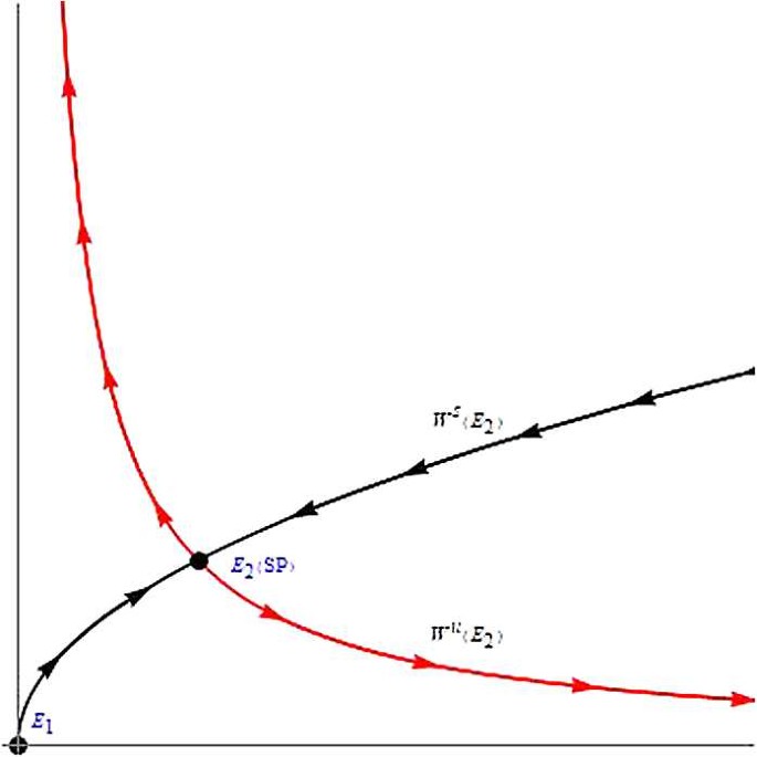

  

  Visual illustration of part (a) of Theorem 7

  In Cases (b)–(e), assume T has at least three fixed points $E_{1}$, $E_{2}$, $E_{3}$, where $E_{1} \prec_{se} E_{2} \prec_{se} E_{3}$, $E_{1}, E_{3}$ are saddle points, and $E_{2}$ is locally asymptotically stable and is the southwest corner of the region $\mathcal{R}$. Assume that the Jacobian $J_{T}(\bar{\mathrm{x}})$ of T evaluated at both $E_{1}$ and $E_{3}$ has real eigenvalues λ, μ such that $0<|\lambda|<1<\mu$ and the eigenspace $E^{\lambda}$ associated with λ is not a coordinate axis. Finally, suppose that the left vertical (resp. bottom horizontal) boundary of $\mathcal{R}$ without $E_{2}$ is $\mathcal {W}^{u}(E_{1})$ (resp. $\mathcal{W}^{u}(E_{3})$).

• (b) In addition to the hypotheses listed above, suppose T has two additional fixed points $E_{4}$ and $E_{5}$ such that $E_{i} \ll_{ne} E_{4} \ll_{ne} E_{5}$ for $i=1,2,3$, $E_{4}$ is a repeller, and $E_{5}$ is a saddle point. Then every solution which starts below (resp. above) the union of the stable manifolds $\mathcal{W}^{s}(E_{3}) \cup\mathcal{W}^{s}(E_{5})$ (resp. $\mathcal{W}^{s}(E_{1}) \cup\mathcal{W}^{s}(E_{5})$) will approach the boundary of the region $\mathcal{R}$. Every solution which starts between the stable manifolds $\mathcal{W}^{s}(E_{1})$ and $\mathcal {W}^{s}(E_{3})$ converges to $E_{2}$. See Fig. 2 for visual illustration.

  Figure 2

  

  Visual illustration of part (b) of Theorem 7

• (c) Assume exactly the hypotheses listed above. Then every solution which starts below (resp. above) the manifold $\mathcal {W}^{s}(E_{3})$ (resp. $\mathcal{W}^{s}(E_{1})$) will approach the boundary of the region $\mathcal{R}$. Every solution which starts between the stable manifolds $\mathcal{W}^{s}(E_{1})$ and $\mathcal{W}^{s}(E_{3})$ converges to $E_{2}$. See Fig. 3 for visual illustration.

  Figure 3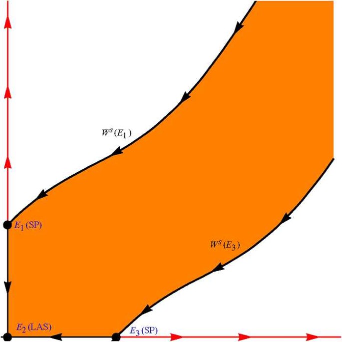

  

  Visual illustration of part (c) of Theorem 7

• (d) In addition to the hypotheses listed above, suppose T has an additional fixed point $E_{4}$ such that $E_{i} \ll_{ne} E_{4}$ for $i=1,2,3$ and $E_{4}$ is nonhyperbolic of unstable type. Assume that no standard basis vector is an eigenvector associated with either of the characteristic values of $E_{4}$. Then there exist continuous, nondecreasing, and invariant curves $\mathcal{C}_{1} ,\mathcal{C}_{2}$ (with $\mathcal{C}_{1}$ above $\mathcal{C}_{2}$) which emanate from $E_{4}$ such that the region between the curves is invariant. The region below (resp. above) the union of invariant curves $\mathcal{W}^{s}(E_{3}) \cup \mathcal{C}_{2}$ (resp. $\mathcal{W}^{s}(E_{1}) \cup \mathcal{C}_{1}$) is invariant, and every solution which starts in either region will approach the boundary of $\mathcal{R}$. If T satisfies condition $(O+)$, for every initial point $(x_{0}, y_{0})$ between $\mathcal{C}_{1}$ and $\mathcal{C}_{2}$, the corresponding solution either converges to $E_{4}$ or approaches the boundary of $\mathcal{R}$. See Fig. 4 for visual illustration.

  Figure 4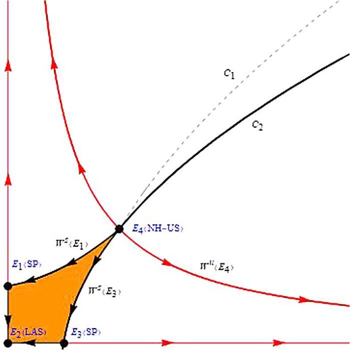

  

  Visual illustration of part (d) of Theorem 7

• (e) In addition to the hypotheses listed above, suppose T has an additional fixed point $E_{4}$ such that $E_{i} \ll_{ne} E_{4}$ for $i=1,2,3$ and $E_{4}$ is a repeller. Assume that no standard basis vector is an eigenvector associated with either of the characteristic values of $E_{4}$. Then there exist continuous, nondecreasing, and invariant curves $\mathcal{C}_{1} ,\mathcal{C}_{2}$ (with $\mathcal{C}_{1}$ above $\mathcal{C}_{2}$) which emanate from $E_{4}$ such that the region between the curves is invariant. The region below (resp. above) the union of invariant curves $\mathcal{W}^{s}(E_{3}) \cup \mathcal{C}_{2}$ (resp. $\mathcal{W}^{s}(E_{1}) \cup \mathcal{C}_{1}$) is invariant, and every solution which starts in either region will approach the boundary of $\mathcal{R}$. If T satisfies condition $(O+)$, for every initial point $(x_{0}, y_{0})$ between $\mathcal{C}_{1}$ and $\mathcal{C}_{2}$, the corresponding solution approaches the boundary of $\mathcal{R}$. See Fig. 5 for visual illustration.

  Figure 5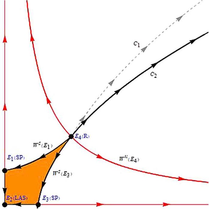

  

  Visual illustration of part (e) of Theorem 7

Proof

• (a) The existence of the global stable and unstable manifolds of the saddle point equilibrium is guaranteed by Theorems 3–6. In any case $\mathcal {W}^{s}(E_{2})$ has endpoints on the boundary of $\mathcal{R}$. In view of Theorem 5, every solution which starts in $\mathcal {W}_{-}$ eventually enters $\operatorname{int}Q_{2}(E_{2})$ and every solution which starts in $\mathcal{W}_{+}$ eventually enters $\operatorname{int}Q_{4}(E_{2})$. If $\vec {x}_{0}=(x_{0},y_{0})\in\mathcal{W}_{+}$, then there exists $m\in\mathbb{N}$ such that $\vec{z}=T^{m}(\vec{x}_{0})\in \operatorname{int}Q_{4}(E_{2})$. Regardless of whether z⃗ is above or below $\mathcal{W}^{u}(E_{2})$, one can find $\vec{u}\in\mathcal{W}^{u}(E_{2})$ such that $\vec{u} \preceq_{se} \vec {z}$. By monotonicity of the map T, this implies that $T^{n}(\vec{u}) \preceq_{se} T^{n}(\vec{z})$ for all $n\in\mathbb{N}$, and so

  $$\lim_{n \to\infty}T^{n}(\vec{u}) \preceq_{se} \lim _{n \to\infty}T^{n}(\vec{z}). $$

  In a similar way the case when the initial point $\vec{x}_{0} \in\mathcal {W}_{-}$ can be handled.

• (b) The existence of the global stable manifolds of $E_{1}$, $E_{3}$, $E_{5}$ and the global unstable manifold of $E_{5}$ is guaranteed by Theorems 3–6; see also [23]. Indeed, by Theorems 3 and 4, both $\mathcal {W}^{s}(E_{1})$ and $\mathcal{W}^{s}(E_{3})$ have endpoints at $E_{4}$, and $\mathcal{W}^{s}(E_{5})$ has endpoints at $E_{4}$ and some point on the boundary of $\mathcal{R}$. Since no other equilibria exist in $Q_{2}(E_{5})\cup Q_{4}(E_{5})$, $\mathcal{W}^{u}(E_{5})$ has endpoints on the boundary of $\mathcal{R}$. Furthermore, the left vertical boundary of the region $\mathcal{R}$ with the exception of $E_{2}$ is the unstable manifold of $E_{1}$ and the bottom horizontal boundary of the region $\mathcal{R}$ with the exception of $E_{2}$ is the unstable manifold of $E_{3}$.

  Let $[\!\![\vec{a},\vec{b}]\!\!]$ be the order interval consisting of all $\vec{c}\in\mathbb{R}^{2}$ such that $\vec {a}\preceq_{ne}\vec{c}\preceq_{ne}\vec{b}$. Consider an arbitrary initial point $\vec{x}_{0}=(x_{0}, y_{0})\in \operatorname{int} [\!\![E_{1}, E_{3} ]\!\!]$. Then there exist some projections onto the unstable manifolds $\mathcal{W}^{u}(E_{1})$ and $\mathcal{W}^{u}(E_{3})$, $P_{y}$ and $P_{x}$, respectively, such that $P_{y} \preceq_{se} \vec{x}_{0} \preceq_{se} P_{x}$, which implies that

  $$ T^{n}(P_{y})\preceq_{se} T^{n}( \vec{x}_{0})\preceq_{se} T^{n}(P_{x}) $$

  for each $n\in\mathbb{N}$. Since $\lim_{n\rightarrow\infty} T^{n}(P_{y})=\lim_{n\rightarrow\infty} T^{n}(P_{x})=E_{2}$, we obtain that $\lim_{n\rightarrow\infty} T^{n}(\vec{x}_{0})=E_{2}$. If $\vec {x}_{0} \in\partial ([\!\![E_{1}, E_{3} ]\!\!])\backslash (\mathcal{W}^{u}(E_{1})\cup\mathcal{W}^{u}(E_{3})\cup E_{2} )$, then $T(\vec{x}_{0})\in \operatorname{int}[\!\![E_{1}, E_{3} ]\!\!]$ and the result follows.

  Now suppose $\vec{x}_{0}\in\mathscr{B}\backslash[\!\![E_{1}, E_{3} ]\!\!]$, where $\mathscr{B}$ denotes the region between the stable manifolds $\mathcal{W}^{s}(E_{1})$ and $\mathcal{W}^{s}(E_{3})$. Then there must exist $\vec{s}_{l}\in\mathcal{W}^{s}(E_{1})$ and $\vec{s}_{u}\in\mathcal {W}^{s}(E_{3})$ such that $\vec{s}_{l}\preceq_{se} \vec{x_{0}}\preceq_{se} \vec {s}_{u}$. But then

  $$T^{n} (\vec{s}_{l} )\preceq_{se} T^{n} (\vec{x_{0}} )\preceq_{se} T^{n} (\vec{s}_{u} ), $$

  and thus $T^{n} (\vec{x_{0}} ) \in[\!\![E_{1}, E_{3} ]\!\!]$ for n sufficiently large, which implies that $\lim_{n\rightarrow\infty}T^{n}(\vec{x_{0}})=E_{2}$.

  Now suppose $\vec{x_{0}}\in \operatorname{int}Q_{4}(E_{5})$. Then there exists $\vec{u}\in \mathcal{W}^{u}(E_{5})$ so that $\vec{u} \preceq_{se} \vec{x_{0}}$, which implies

  $$T^{n} (\vec{u} )\preceq_{se} T^{n} ( \vec{x}_{0} ), $$

  and thus the solution approaches the boundary of the region $\mathcal {R}$. The treatment is similar for $\vec{x}_{0}\in \operatorname{int}Q_{2}(E_{5})$.

  Suppose $\vec{x}_{0}\in Q_{1}(E_{5})$. Without loss of generality suppose $\vec{x}_{0}$ is to the right of $\mathcal{W}^{s}(E_{5})$ (otherwise the treatment is analogous) so that there exists some $\vec{p}\in\mathcal {W}^{s}(E_{5})$ such that $\vec{p}\preceq_{se} \vec{x}_{0}$. We claim that there exists some n such that $T^{n}(\vec{x}_{0})\in \operatorname{int}Q_{4}(E_{5})$. Certainly for any n it is the case that $T^{n}(\vec{p})\preceq_{se} T^{n}(\vec{x}_{0})$. For a contradiction suppose $T^{n}(\vec{x}_{0})\rightarrow E_{5}$ as $n\rightarrow\infty$. But then for some n, $T^{n}(\vec{x}_{0})\in \mathcal{W}^{s}_{\footnotesize\mbox{loc}}(E_{5})$, the local stable manifold tangential to the eigenspace $E^{\lambda}$. Since in a small neighborhood of $E_{5}$ we have that $\mathcal{W}^{s}_{\footnotesize\mbox{loc}}(E_{5})\subseteq\mathcal{W}^{s}(E_{5})$, we now have the relation $T^{n}(\vec{p})\preceq_{se} T^{n}(\vec{x}_{0})$, but any points on this invariant curve are not comparable with respect to the southeast ordering. By continuity of T the only finite points to which any solution may converge are fixed points, and therefore it must be the case that eventually the solution enters $\operatorname{int}Q_{4}(E_{5})$.

  Suppose $\vec{x}_{0}\in[\!\![E_{2}, E_{5}]\!\!]\backslash [\!\![E_{2}, E_{4}]\!\!]$. In any case we can compare $\vec{x}_{0}$ to a point on $\mathcal{W}^{s}(E_{5})$ and show using a similar argument as that used above that the corresponding solution must enter either $\operatorname{int} Q_{4}(E_{5})$ or $\operatorname{int}Q_{2}(E_{5})$ (in which case we can apply the previous results to establish the long-term behavior of the solution).

  Finally suppose $\vec{x}_{0}\in[\!\![E_{2}, E_{4}]\!\!]\backslash \overline{\mathscr{B}}$. By comparing $\vec{x}_{0}$ to some point on either $\mathcal{W}^{s}(E_{3})$ or $\mathcal{W}^{s}(E_{1})$ as appropriate, we may utilize a similar argument as before to deduce that the corresponding solution cannot converge to $E_{3}$ or $E_{1}$. Thus there exists some $n\in\mathbb{N}$ such that $T^{n}(\vec{x}_{0})\in \operatorname{int} Q_{4}(E_{5})$ (or $T^{n}(\vec{x}_{0})\in \operatorname{int}Q_{2}(E_{5})$), and we can apply the results of the previous case to complete the proof.

• (c) The proofs used to show that the region between the stable manifolds $\mathcal{W}^{s}(E_{1})$ and $\mathcal{W}^{s}(E_{3})$ is the basin of attraction of $E_{2}$ and that solutions with initial conditions starting outside this region will approach the boundary of the region are similar to those provided in case (b) and will be omitted.

• (d) The proof used to show that the region between the stable manifolds $\mathcal{W}^{s}(E_{1})$ and $\mathcal{W}^{s}(E_{3})$ is the basin of attraction of $E_{2}$ is the same as in case (b) and will be omitted. In view of the main result in [23] there exists a most unstable manifold $\mathcal {W}^{u}_{\mbox{max}}(E_{4})$, which is the graph of a decreasing function passing through $E_{4}$, which at $E_{4}$ is tangent to the eigenspace that corresponds to the largest (in absolute value) eigenvalue. The existence of the invariant curves $\mathcal{C}_{1} ,\mathcal{C}_{2}$ is guaranteed by Theorem 2 applied to the open rectangular region $\mathcal{R}'=\operatorname{int}\mathcal{R}$, in which T has only the interior fixed point $E_{4}$. The endpoints $q_{1}$ and $q_{2}$ of the full curves $\mathcal{C}_{1}$ and $\mathcal{C}_{2}$, respectively, should coincide with the fixed points $E_{1}$ and $E_{3}$ on the boundary. The proofs that nth iterates of points which start in the invariant region below $\mathcal{W}^{s}(E_{3}) \cup \mathcal{C}_{2}$ (resp. above $\mathcal{W}^{s}(E_{1}) \cup \mathcal{C}_{1}$) are approaching the boundary of the region $\mathcal{R}$ are similar to those provided in case (b); also, see Theorem 2 (ii). If an initial point $\vec{x}_{0}=(x_{0}, y_{0})\in Q_{1}(E_{4})$ is between $\mathcal {C}_{1}$ and $\mathcal{C}_{2}$, then there exist points $\vec{c}_{i} \in \mathcal{C}_{i}, i=1,2$, such that $\vec{c}_{1} \preceq_{se} \vec{x}_{0} \preceq_{se} \vec{c}_{2}$. In view of Corollary 1, if T additionally satisfies condition $(O+)$, then the solution approaches the boundary of the region or $T^{n} (\vec{x}_{0} ) \to E_{4}$ as $n \to\infty$.

• (e) The proof for this case is analogous to that provided in case (d) and will be omitted. Note that if T satisfies condition (O+), then every solution with initial point $\vec{x_{0}}=(x_{0},y_{0})\in Q_{1}(E_{4})$ between the curves $\mathcal{C}_{1}$ and $\mathcal{C}_{2}$ must approach the boundary of the region since in this case $E_{4}$ is a repeller and has a trivial basin of attraction.

 □

In the case of Equation (4) we have the following results which are direct applications of Theorem 7. See [10] for similar results.

Theorem 8

Consider Equation (4) on a rectangular region $\mathcal {R}=[a,b)\times[a,b)$, where $b\leq\infty$. Assume that f is decreasing in the first variable and increasing in the second variable on $(a, b)^{2}$ such that f is $C^{2}$ in a neighborhood of any fixed point.

• (a) Assume that Equation (4) has one saddle equilibrium point $\bar {x}>a$ and that a is either a repelling (or nonhyperbolic) equilibrium point or a singular point of $\mathcal{R}$. If Equation (4) has no minimal period-two solutions, then every nonconstant solution which starts off the stable manifold $\mathcal{W}^{s}((\bar {x},\bar {x}))$ will approach the boundary of the region $\mathcal{R}$.

  In Cases (b)–(e), assume that Equation (4) has a locally asymptotically stable equilibrium point a and the unique minimal period-two solution $\{a,p,a,p,\ldots\}$, with $p>a$, such that $P_{1}=(a,p)$ and $P_{2}=(p,a)$ are saddle points. Assume further that the Jacobian $J_{T^{2}}(\bar{\mathrm{x}})$ of $T^{2}$, where T is the map corresponding to Equation (4), evaluated at both $P_{1}$ and $P_{2}$ has real eigenvalues λ, μ such that $0<|\lambda |<1<\mu$ and the eigenspace $E^{\lambda}$ associated with λ is not a coordinate axis. Finally, suppose that $\mathcal{W}^{u}(P_{1})=\{ (x,y):x=a,y\neq a\}$ and $\mathcal{W}^{u}(P_{2})=\{(x,y):y=a,x\neq a\}$.

• (b) In addition to the hypotheses listed above, assume that Equation (4) has two additional equilibrium points $\bar {x}_{2},\bar {x}_{1}$ such that $\bar {x}_{2}>\bar {x}_{1}>a$, $\bar {x}_{1}$ is a repeller, and $\bar {x}_{2}$ is a saddle point. Then every solution which starts between the stable manifolds $\mathcal{W}^{s}(P_{1})$ and $\mathcal{W}^{s}(P_{2})$ converges to $(a, a)$ while every solution which starts below $\mathcal{W}^{s}((\bar {x}_{2},\bar {x}_{2})) \cup\mathcal{W}^{s}(P_{2})$ (resp. above $\mathcal{W}^{s}((\bar {x}_{2},\bar {x}_{2})) \cup\mathcal {W}^{s}(P_{1})$) is approaching the boundary of the region $\mathcal{R}$.

• (c) Assume exactly the hypotheses listed above. Then every solution which starts between the stable manifolds $\mathcal{W}^{s}(P_{1})$ and $\mathcal{W}^{s}(P_{2})$ converges to $(a, a)$ while every solution which starts below $\mathcal{W}^{s}(P_{2})$ (resp. above $\mathcal{W}^{s}(P_{1})$) is approaching the boundary of the region $\mathcal{R}$.

• (d) In addition to the hypotheses listed above, assume that Equation (4) has an additional equilibrium point x̄ such that $\bar {x}>a$ and x̄ is nonhyperbolic of unstable type. Assume that no standard basis vector is an eigenvector associated with either of the eigenvalues of the Jacobian $J_{T^{2}}(\bar{\mathrm{x}})$ evaluated at $(\bar {x},\bar {x})$. Then there exist two continuous and nondecreasing curves $\mathcal{C}_{1}$ and $\mathcal{C}_{2}$ (with $\mathcal {C}_{1}$ above $\mathcal{C}_{2}$) which start at $(\bar {x},\bar {x})$ and serve as the boundary of the region containing the basin of attraction of $(\bar {x},\bar {x})$. Every solution which starts between the stable manifolds $\mathcal{W}^{s}(P_{1})$ and $\mathcal{W}^{s}(P_{2})$ converges to $(a, a)$, while every solution which starts below $\mathcal{W}^{s}(P_{2}) \cup \mathcal{C}_{2}$ (resp. above $\mathcal{W}^{s}(P_{1}) \cup \mathcal {C}_{1}$) is approaching the boundary of the region $\mathcal{R}$. Every solution which starts between $\mathcal{C}_{1}$ and $\mathcal{C}_{2}$ converges to $(\bar {x},\bar {x})$ or approaches the boundary of the region.

• (e) In addition to the hypotheses listed above, assume that Equation (4) has an additional equilibrium point x̄ such that $\bar {x}>a$ and x̄ is a repeller. Assume that no standard basis vector is an eigenvector associated with either of the eigenvalues of the Jacobian $J_{T^{2}}(\bar{\mathrm{x}})$ evaluated at $(\bar {x},\bar {x})$. Then there exist two continuous and nondecreasing curves $\mathcal{C}_{1}$ and $\mathcal{C}_{2}$ (with $\mathcal{C}_{1}$ above $\mathcal{C}_{2}$) which start at $(\bar {x},\bar {x})$. Every solution which starts between the stable manifolds $\mathcal{W}^{s}(P_{1})$ and $\mathcal {W}^{s}(P_{2})$ converges to $(a, a)$, while every solution which starts below $\mathcal{W}^{s}(P_{2}) \cup \mathcal{C}_{2}$ (resp. above $\mathcal {W}^{s}(P_{1}) \cup \mathcal{C}_{1}$) is approaching the boundary of the region $\mathcal{R}$. Every solution which starts between $\mathcal {C}_{1}$ and $\mathcal{C}_{2}$ approaches the boundary of the region.

Proof

In all cases recall that the applicability of Theorem 7 to a map T requires the nonexistence of minimal period-two solutions. Since we seek to apply the results of this theorem to $T^{2}$, where T is the map corresponding to Equation (4), we must rule out the possibility of minimal period-four solutions for Equation (4). However, realize that Theorem 1 specifically precludes the existence of periodic solutions of prime period greater than two.

• (a) In view of Remark 2 the second iterate $T^{2}$ of the map T associated with Equation (4) is strongly competitive on $(a,b)^{2}$. Applying Theorem 7 part (a) to $T^{2}$, we complete the proof.

• (b) In view of Remark 2 the second iterate $T^{2}$ of the map T associated with Equation (4) is strongly competitive and has five equilibrium points $E_{1}=P_{1}$, $E_{2}=(a,a)$, $E_{3}=P_{2}$, $E_{4}=(\bar {x}_{1},\bar {x}_{1})$, and $E_{5}=(\bar {x}_{2},\bar {x}_{2})$. Applying Theorem 7 part (b) to $T^{2}$, we conclude that

  $$\lim_{n\rightarrow\infty} T^{2n}\bigl((x_{0}, y_{0})\bigr)=E_{2} $$

  for every $(x_{0}, y_{0})$ between the stable manifolds $\mathcal {W}^{s}(P_{1})$ and $\mathcal{W}^{s}(P_{2})$. Furthermore, we also have that

  $$ \lim_{n\rightarrow\infty} T^{2n+1}\bigl((x_{0}, y_{0})\bigr)=\lim_{n\rightarrow\infty}T \bigl(T^{2n} \bigl((x_{0}, y_{0}) \bigr) \bigr)=T \Bigl(\lim _{n\rightarrow\infty} T^{2n} \bigl((x_{0}, y_{0}) \bigr) \Bigr)=T(E_{2})=E_{2}, $$

  where we utilize continuity of the map T. Consequently, $\lim_{n\rightarrow\infty} T^{n}((x_{0}, y_{0}))=E_{2}$. The remaining conclusions follow from Theorem 7 part (b).

• (c)–(e) The proofs of parts (c), (d), and (e) follow in a similar way by using the same reasoning as in parts (a) and (b). For parts (d) and (e), make the observation that condition (O+) is automatically satisfied for the second iterate of the map T corresponding to Equation (4); see [17, 18].

 □

Remark 4

As shown in [19], the curves $\mathcal{C}_{1}$ and $\mathcal {C}_{2}$ may coincide on one or both sides of the fixed point. Different global dynamic scenarios for competitive or cooperative maps and corresponding difference equations were established in the cases when these maps have a finite or infinite number of period-two solutions in [2, 4, 19].

Remark 5

Some special cases of Theorems 7 and 8 have appeared in a number of papers. For example, the global dynamics of the system

$$x_{n+1}=\frac{x_{n}}{a+y_{n}}, \qquad y_{n+1}=\frac{y_{n}}{b+ x_{n}}, \quad n=0,1,\ldots, $$

where $a,b \in(0,1)$ and $x_{0},y_{0} \in[0, \infty)$, as studied in [6], follows from Theorem 7 case (a). Furthermore, several cases of the global dynamics of the system

$$x_{n+1}=\frac{ax_{n}^{2}}{1+ x_{n}^{2} + cy_{n}}, \qquad y_{n+1}=\frac{b y_{n}^{2}}{1+ d x_{n} + y_{n}^{2}}, \quad n=0,1,\ldots, $$

where $a,b,c,d \in(0,\infty)$ and $x_{0},y_{0} \in[0, \infty)$, as studied in [3], follow from Theorem 7 cases (a)–(d).

The global dynamics of the difference equations

$$x_{n+1}=\frac{x_{n-1}(x_{n} +\gamma)}{x_{n}(x_{n}+Bx_{n-1})}, \quad n=0,1,\ldots, $$

where $B, \gamma>0$ and $B<4 \gamma+1$, and

$$x_{n+1}=\frac{x_{n}^{2} + \beta x_{n} x_{n-1} +\gamma x_{n-1}}{x_{n}^{2}}, \quad n=0,1,\ldots, $$

where $\beta, \gamma>0, \beta+\gamma\geq1, 4\gamma+ 2 \beta+\beta^{2} >3$, is described by Theorem 8 case (a).

The global dynamics of the difference equation

$$x_{n+1}=\frac{x_{n-1}^{2}}{b x_{n}x_{n} + c x_{n-1}^{2} + f}, \quad n=0,1,\ldots, $$

where $b,c,f \geq0$ and $b+c+f>0$, is described by Theorem 8 cases (a)–(d) for several regions of parameters.

Finally, the global dynamics of the well-known difference equations

$$x_{n+1}= a+\frac{x_{n-1}}{x_{n}}, \quad n=0,1,\ldots, $$

where $a \in(0,1)$, and

$$x_{n+1}=\frac{p+ q x_{n-1}}{1+x_{n}}, \quad n=0,1,\ldots, $$

where $p>0,q >1$, is described by Theorem 8 case (a). See [12], pp. 60–64 and pp. 89–91 of [15], and the references therein.

It is worth noticing that case (e) in both Theorems 7 and 8 has been identified for the first time in the case of Equation (1).

4 Case study: Equation (1)

In this section we apply the results of Theorem 8 to the study of the global dynamics of Equation (1). We begin by investigating the existence and local stability of equilibria and periodic solutions.

4.1 Equilibrium solutions of Equation (1)

An equilibrium point x̄ of Equation (1) satisfies

$$ a\bar {x}^{3}+(d-C)\bar {x}^{2}+(f-E)\bar {x}=0. $$

(6)

In the case when $f>0$, it is clear that Equation (6) always has the zero equilibrium. The following cases will investigate the existence of any remaining positive equilibrium points.

4.1.1 Case 1 ($af>0$):

When $f>0$ and $a>0$, denote by $\bar {x}_{+}$ and $\bar {x}_{-}$ the two possibly remaining positive equilibria:

$$ \bar {x}_{\pm}=\frac{(C-d)\pm\sqrt{(C-d)^{2}-4a(f-E)}}{2a}. $$

(7)

Let $R=(C-d)^{2}-4a(f-E)$. A routine checking will find the parametric conditions under which the above solutions $\bar {x}_{+}$ and $\bar {x}_{-}$ are both real and nonnegative. Tables 1 and 2 summarize the values of parameters for which Equation (1) has one, two, or three equilibrium points and possibly period-two solutions (the existence of which we will investigate in Sect. 4.3).

Table 1 Existence of equilibria and period-two solutions for $a>0$, $f>0$, $C>0$

Table 2 Existence of equilibria and period-two solutions for $a>0$, $f>0$, $C=0$

4.1.2 Case 2 ($af=0$):

When $f>0$ but $a=0$, notice that Equation (6) reduces to

$$ \bar {x}\bigl((d-C)\bar {x}+(f-E) \bigr)=0, $$

which has the isolated solutions $\bar {x}_{0}=0$ and possibly $\bar {x}_{+}=\frac{f-E}{C-d}$. Existence of equilibria is summarized in Table 3.

Table 3 Existence of equilibria and period-two solutions for $a=0$, $f>0$

When $a>0$ and $f=0$, Equation (6) becomes

$$ \bar {x}\bigl(a\bar {x}^{2}+(d-C)\bar {x}-E \bigr)=0, $$

and since necessarily $\bar {x}\neq0$ in this case, Descartes’ Rule of Signs yields that there may exist at most one positive fixed point $\bar {x}_{+}>0$. See Table 4 for a summary of the parametric conditions under which an equilibrium point exists.

Table 4 Existence of equilibria for $a>0$, $f=0$

In the case $a=f=0$ the solutions of Equation (6) must satisfy

$$ \bar {x}\bigl((d-C)\bar {x}-E \bigr)=0. $$

Since we must have $\bar {x}>0$, this equation has the isolated solution $\bar {x}_{+}=\frac{E}{d-C}$ only when $d>C$ and $E>0$. All remaining subcases may be summarized in Table 5.

Table 5 Existence of equilibria for $a=0$, $f=0$

4.2 Local stability analysis of the equilibrium solutions

Define the function g such that

$$ g(u,v)=\frac{Cv^{2}+ Ev}{a u^{2}+d u+f} $$

so that Equation (1) becomes $x_{n+1}=g(x_{n},x_{n-1})$. The partial derivatives of g are given by

$$ g_{u}(u,v)=\frac{-(Cv^{2}+Ev)(2au+d)}{(au^{2}+du+f)^{2}}\quad \mbox{and}\quad g_{v}(u,v)=\frac{2Cv+E}{au^{2}+du+f}. $$

The characteristic equation of the linearization of Equation (1) about x̄ is $\lambda^{2}=P\lambda+Q$, where $P=g_{u}(\bar {x},\bar {x})$ and $Q=g_{v}(\bar {x},\bar {x})$. Using Equation (6), this becomes

$$ \lambda^{2}=\frac{-\bar {x}(2a\bar {x}+d)}{a\bar {x}^{2}+d\bar {x}+f}\lambda+ \frac {2C\bar {x}+E}{a\bar {x}^{2}+d\bar {x}+f}. $$

(8)

Lemma 1

The zero equilibrium $\bar {x}_{0}=0$, which exists whenever $f>0$, has the following stability:

$$\bar {x}_{0}=0 \textit{ is } \textstyle\begin{cases} \textit{locally asymptotically stable} & \textit{if } E< f,\\ \textit{a repeller} &\textit{if }E>f,\\ \textit{nonhyperbolic }(\textit{resonant }(1,-1)\textit{ type}) &\textit{if } E=f. \end{cases} $$

Proof

Notice that, evaluated at $\bar {x}_{0}$, $P=0$ and $Q=\frac{E}{f}$. Using Theorem 2.13 of [16], the first two results of the claim are immediate by checking the necessary inequalities.

If $E=f$, then the characteristic equation of the linearized equation of Equation (1) (given in Equation (8)) is $\lambda^{2}=1$ and hence $\lambda_{1}=1$, $\lambda_{2}=-1$ so that $\bar {x}_{0}$ is nonhyperbolic of resonant type $(1, -1)$. □

4.2.1 Case 1 ($a f>0$):

Lemma 2

Assume that $af>0$.

• (a) If $C>d$, $f>E$, and $(C-d)^{2}=4a(f-E)$, then $\bar {x}_{\pm }=\frac{C-d}{2a}$ is a nonhyperbolic equilibrium point of unstable type.

• (b) Suppose one of the following conditions holds:

  • 1. $f< E$,

  • 2. $C>d$, $f=E$,

  • 3. $C>d$, $f>E$, $(C-d)^{2}>4a(f-E)$.

  Then the positive equilibrium $\bar {x}_{+}$ is a saddle point.

• (c) If $C>d$, $f>E$, and $(C-d)^{2}>4a(f-E)$, then $\bar {x}_{-}$ is a repeller.

Proof

• (a) Notice that, for $\bar {x}\neq0$, we have the following:

  $$\begin{aligned} \vert P \vert -1+Q&=\frac{\bar {x}(2a\bar {x}+d)-(a\bar {x}^{2}+d\bar {x}+f)+2C\bar {x}+E}{a\bar {x}^{2}+d\bar {x}+f} \\ &=\frac{2a\bar {x}^{2}+d\bar {x}-(a\bar {x}^{2}+(d-C)\bar {x}+(f-E))+C\bar {x}}{a\bar {x}^{2}+d\bar {x}+f} \\ &=\frac{2a\bar {x}^{2}+d\bar {x}+C\bar {x}}{a\bar {x}^{2}+d\bar {x}+f}>0, \end{aligned}$$

  (9)

  and

  $$\begin{aligned} \vert P \vert +1-Q&=\frac{\bar {x}(2a\bar {x}+d)+(a\bar {x}^{2}+d\bar {x}+f)-(2C\bar {x}+E)}{a\bar {x}^{2}+d\bar {x}+f} \\ &=\frac{2a\bar {x}^{2}+d\bar {x}+(a\bar {x}^{2}+(d-C)\bar {x}+(f-E))-C\bar {x}}{a\bar {x}^{2}+d\bar {x}+f} \\ &=\frac{\bar {x}(2a\bar {x}+(d-C))}{a\bar {x}^{2}+d\bar {x}+f}. \end{aligned}$$

  (10)

  From Equation (10) it is clear that, for $\bar {x}_{\pm }=\frac{C-d}{2a}$, $|P|+1-Q=0$, and hence this equilibrium is indeed nonhyperbolic. Using the equilibrium equation and the fact that $2a\bar {x}_{\pm}+d=C$, notice that the characteristic equation (8) becomes

  $$\begin{aligned} &\lambda^{2}=\frac{-\bar {x}(2a\bar {x}+d)}{a\bar {x}^{2}+d\bar {x}+f}\lambda+\frac {2C\bar {x}+E}{a\bar {x}^{2}+d\bar {x}+f}\\ &\quad \iff\quad \lambda^{2}+\frac{C\bar {x}}{C\bar {x}+E}\lambda-\frac{2C\bar {x}+E}{C\bar {x}+E}=0 \\ &\quad \iff\quad (\lambda-1) \biggl(\lambda+\frac{2C\bar {x}+E}{C\bar {x}+E} \biggr)=0. \end{aligned}$$

  Since $\lambda_{1}=1$ and $\lambda_{2}=-\frac{2C\bar {x}+E}{C\bar {x}+E}<-1$, this nonhyperbolic equilibrium point is of the unstable type.

• (b) Note that in all but the last case $\bar {x}_{+}$ is the unique positive equilibrium. It is clear from Equation (10) that $|P|+1-Q>0$ if and only if $2a\bar {x}>C-d$. However, by definition in Equation (7) we have that

  $$2a\bar {x}_{+}=(C-d)+\sqrt{(C-d)^{2}-4a(f-E)}>(C-d). $$

  Therefore $|P|>1-Q>-|P|\iff|1-Q|<|P|$, and thus by Theorem 2.13 of [16], $\bar {x}_{+}$ is a saddle point for all values of parameters for which it exists.

• (c) Since

  $$2a\bar {x}_{-}=(C-d)-\sqrt{(C-d)^{2}-4a(f-E)}< C-d, $$

  by Equation (10) we have that $|P|+1-Q<0$ and hence $|P|<|1-Q|$. Now

  $$\begin{aligned} \vert Q \vert >1& \quad \iff\quad 2C\bar {x}_{-}+E>a\bar {x}_{-}^{2}+d \bar {x}_{-}+f \\ & \quad \iff\quad C\bar {x}_{-}> a\bar {x}_{-}^{2}+(d-C) \bar {x}_{-}+(f-E) \\ & \quad \iff\quad C\bar {x}_{-}^{2}>0, \end{aligned}$$

  after we use Equation (6). Thus by Theorem 2.13 of [16], $\bar {x}_{-}$ is indeed a repeller.

 □

4.2.2 Case 2 ($af=0$):

Lemma 3

• (a) Suppose $a=0$ and $f>0$.

  • 1. If $C< d$ and $f< E$, then $\bar {x}_{+}$ is a saddle point.

  • 2. If $C>d$ and $f>E$, then $\bar {x}_{+}$ is a repeller.

  • 3. If $C=d$ and $f=E$, then every point $\bar {x}> 0$ is a nonhyperbolic equilibrium of unstable type.

• (b) If $a>0$, $f=0$, and either $E>0$ or ($C>d$ and $E=0$), then $\bar {x}_{+}$ is a saddle point.

• (c) Suppose $a=f=0$.

  • 1. If $C< d$ and $E>0$, then $\bar {x}_{+}$ is a saddle point.

  • 2. If $C=d$ and $E=0$, then any $\bar {x}>0$ is a nonhyperbolic equilibrium of unstable type.

Proof

• (a) By Equation (10), we have that

  $$\begin{aligned} \vert P \vert +1-Q&=\frac{\bar {x}(d-C)}{d\bar {x}+f}\\ &=\frac{E-f}{d\bar {x}+f} \textstyle\begin{cases} >0, & E>f,\\ < 0, & E< f,\\ =0, & E=f. \end{cases}\displaystyle \end{aligned}$$

  By Equation (9) we have that $|P|-1+Q>0$. In the case when $C>d$, we can also check immediately that $|Q|>1$. Thus when $E>f$ and $C< d$, $\bar {x}_{+}$ is a saddle point, and when $E< f$ and $C>d$, $\bar {x}_{+}$ is a repeller, which establishes Cases 1 and 2. In the nonhyperbolic case when $E=f$ and $C=d$, each point $\bar {x}> 0$ is an equilibrium point and the characteristic equation (8) reduces to

  $$ \lambda^{2}+\frac{d\bar {x}}{d\bar {x}+f}\lambda-\frac{2d\bar {x}+f}{d\bar {x}+f}=0\quad \iff\quad (\lambda-1) \biggl(\lambda+\frac{2d\bar {x}+f}{d\bar {x}+f} \biggr)=0. $$

  But then $\lambda_{1}=1$ and $\lambda_{2}<-1$ so that each nonhyperbolic equilibrium is of the unstable type.

  Thus we have verified Case 3, and the proof is complete.

• (b) The result immediately follows from Equations (9) and (10).

• (c)

  • 1. When $d>C$ and $E>0$, Equation (10) reduces to

    $$\vert P \vert +1-Q=\frac{E}{d\bar {x}}>0, $$

    and coupling this result with Equation (9) shows that $\bar {x}_{+}$ is a saddle point.

  • 2. If $d=C$ and $E=0$, Equation (10) implies that any $\bar {x}>0$ is nonhyperbolic. Equation (8) reduces to

    $$ \lambda^{2}+\lambda-2=0, $$

    whence we deduce that $\lambda_{1}=1$ and $\lambda_{2}=-2$, so a nonhyperbolic equilibrium $\bar {x}>0$ is of the unstable type in this case.

 □

4.3 Periodic solutions

Lemma 4

Consider Equation (1).

• (a) There exists no strictly positive minimal period-two solution to Equation (1).

• (b) If $f>E$ and $C>0$, Equation (1) possesses the minimal period-two solution $\{0,\frac{f-E}{C},0,\frac{f-E}{C},\ldots\}$. If $C=0$ and $f=E$, then every point on the positive x- or y-axis is a period-two point.

Proof

• (a) Suppose on the contrary that there exists a strictly positive periodic solution $\{\phi,\psi,\phi,\psi,\ldots\}$ with $\phi\neq\psi$. Now ϕ and ψ satisfy:

  $$\begin{aligned} &\phi= g(\psi,\phi)=\frac{C\phi^{2}+E\phi}{a\psi^{2}+d\psi+f}, \\ &\psi= g(\phi,\psi)=\frac{C\psi^{2}+E\psi}{a\phi^{2}+d\phi+f}, \end{aligned}$$

  which together imply

  $$\begin{aligned} &(C\psi+E) \bigl(a\psi^{2}+d\psi+f\bigr)-(C\phi+E) \bigl(a \phi^{2}+d\phi+f\bigr)=0, \\ &\quad \iff\quad (\psi-\phi)\bigl[aC\bigl( \psi^{2}+\psi\phi+\phi^{2}\bigr)+(Cd+aE) (\psi+\phi )+(Cf+dE) \bigr]=0. \end{aligned}$$

  (11)

  Since $a+d>0$, $a+C>0$, and $C+E>0$, it is clear that the latter factor of Equation (11) is strictly positive in any case, so we deduce that $\psi=\phi$, a contradiction. Thus no positive minimal period-two solution exists to Equation (1).

• (b) In light of (a) there exists no interior period-two solution of Equation (1). Therefore, suppose there exists a periodic solution $\{\phi,\psi,\phi,\psi,\ldots\}$ with $\phi\neq\psi$ and $\phi+\psi>0$. Without loss of generality, we may set $\phi=0$. Now

  $$\psi= g(0,\psi)=\frac{C\psi^{2}+E\psi}{f}\quad \iff\quad f-E= C\psi, $$

  whence the result follows. Notice that if $C=0$ and $f=E$, then any $\psi>0$ will satisfy the above equation, establishing the second claim.

 □

The following result gives the relation between the equilibria and period-two solutions.

Lemma 5

• (a) If $af>0$, $C>d$, $f>E$, and $(C-d)^{2}\geq4a(f-E)$, $\bar {x}_{-}$ (or $\bar {x}_{\pm}$) is defined as in Equation (7), and $\psi=\frac{f-E}{C}$, then $\psi<\bar {x}_{-}$ (or $\psi<\bar {x}_{\pm}$).

• (b) If $a=0$, $f>0$, $C>d$, and $f>E$, then $\psi<\bar {x}_{+}$.

Proof

• (a) We need to check the following inequality:

  $$\begin{aligned} &\frac{f-E}{C}< \frac{(C-d)-\sqrt{(C-d)^{2}-4a(f-E)}}{2a} \\ &\quad \iff\quad \sqrt {(C-d)^{2}-4a(f-E)}< (C-d)- \frac{2a(f-E)}{C}. \end{aligned}$$

  (12)

  Notice that the right-hand side of Inequality (12) is positive since $a>0$:

  $$\frac{C(C-d)-2a(f-E)}{C}>\frac{(C-d)^{2}-4a(f-E)}{C}\geq0. $$

  If $(C-d)^{2}=4a(f-E)$ the result immediately follows. If $(C-d)^{2}>4a(f-E)$, we may square both sides of Inequality (12) to obtain

  $$\begin{aligned} &(C-d)^{2}-4a(f-E)< \biggl((C-d)-\frac{2a(f-E)}{C} \biggr)^{2} \\ &\quad \iff\quad 0< C^{2}-C(C-d)+a(f-E)=dC+a(f-E), \end{aligned}$$

  which is always true by assumption. Thus indeed $\psi <\bar {x}_{-}$.

• (b) In this case $\bar {x}_{+}=\frac{f-E}{C-d}$, so $\psi<\bar {x}_{+}$ by definition since necessarily $d>0$.

 □

4.4 Local stability analysis of the period-two solution

Lemma 6

Consider Equation (1).

• (a) If $f>E$ and $C>0$, the period-two points $(\frac{f-E}{C},0)$ and $(0,\frac{f-E}{C})$ are saddle points.

• (b) If $C=0$ and $f=E$, then each point on the positive x- or y-axis is a nonhyperbolic period-two point of stable type.

Proof

Using the substitution $x_{n-1}=u_{n}$, $x_{n}=v_{n}$, Equation (1) becomes

$$\begin{aligned} &u_{n+1}=v_{n}, \\ &v_{n+1}=\frac{Cu_{n}^{2}+Eu_{n}}{av_{n}^{2}+dv_{n}+f}. \end{aligned}$$

The corresponding map T is thus given by

$$T \begin{pmatrix} u\\ v \end{pmatrix}= \begin{pmatrix} v\\ g(v,u) \end{pmatrix}. $$

The second iteration $T^{2}$ of the map is given by

$$T^{2} \begin{pmatrix} u\\ v \end{pmatrix} = T\begin{pmatrix} v\\ g(v,u) \end{pmatrix} = \begin{pmatrix} g(v,u)\\ g(g(v,u),v) \end{pmatrix}\stackrel{\mathrm{set}}{=}\begin{pmatrix} F(u,v)\\ G(u,v) \end{pmatrix}, $$

where

$$F(u,v)=g(v,u)=\frac{Cu^{2}+Eu}{av^{2}+dv+f},\qquad G(u,v)=\frac{Cv^{2}+Ev}{aF^{2}(u,v)+dF(u,v)+f}. $$

Notice that the map $T^{2}$ is strongly competitive. The Jacobian of $T^{2}$ is given by

$$ \begin{pmatrix} \frac{\partial F}{\partial u} & \frac{\partial F}{\partial v}\\ \frac{\partial G}{\partial u} & \frac{\partial G}{\partial v} \end{pmatrix}, $$

where

$$\begin{aligned} \frac{\partial F}{\partial u}&=\frac{2Cu+E}{av^{2}+dv+f}, \\ \frac{\partial F}{\partial v}&=\frac {-(Cu^{2}+Eu)(2av+d)}{(av^{2}+dv+f)^{2}}, \\ \frac{\partial G}{\partial u}&=\frac{-(Cv^{2}+Ev)(2aF(u,v)+d)\cdot\frac {\partial F}{\partial u}}{(aF^{2}(u,v)+dF(u,v)+f)^{2}}, \\ \frac{\partial G}{\partial v}&=\frac {(2Cv+E)(aF^{2}(u,v)+dF(u,v)+f)-(2aF(u,v)+d)\cdot\frac{\partial F}{\partial v}\cdot(Cv^{2}+Ev)}{(aF^{2}(u,v)+dF(u,v)+f)^{2}}. \end{aligned}$$

Notice that if Equation (1) has the period-two solution $\{0,\psi,0,\psi,\ldots\}$ for $\psi>0$, then $(0,\psi)$ and $(\psi,0)$ are both fixed points of $T^{2}$. The Jacobian of $T^{2}$ at the point $(0,\psi)$ has the following form:

$$\mbox{Jac}_{T^{2}} \begin{pmatrix} 0\\ \psi \end{pmatrix}= \begin{pmatrix} \frac{E}{a\psi^{2}+d\psi+f} & 0\\ -\frac{Ed\psi}{f(a\psi^{2}+d\psi+f)} & \frac{2C\psi+E}{f} \end{pmatrix}, $$

which has eigenvalues $\lambda_{1}=\frac{E}{a\psi^{2}+d\psi+f}$ and $\lambda_{2}=\frac{2C\psi+E}{f}$.

• (a) If $f>E$ and $C>0$, then $\psi=\frac{f-E}{C}$. Therefore

  $$\begin{aligned} \vert \lambda_{1} \vert < 1&\quad \iff\quad E< a\psi^{2}+d\psi+f, \quad \mbox{and} \\ \vert \lambda_{2} \vert >1&\quad \iff\quad 2C\psi+E>f\quad \iff\quad 2f-2E+E>f\quad \iff\quad f>E. \end{aligned}$$

  Moreover, one can check that no eigenvector corresponding to $\lambda _{1}$ is aligned with a coordinate axis if $E>0$ and $d>0$. A similar calculation will hold for $(\frac{f-E}{C},0)$. Thus the minimal period-two points are indeed saddle points.

• (b) The eigenvalues of the Jacobian of $T^{2}$ evaluated at the point $(0,\psi )$ are given above for an arbitrary $\psi>0$. But since $\lambda_{2}=\frac {2C\psi+E}{f}$, by our hypothesis $\lambda_{2}=1$ and $\lambda_{1}=\frac {E}{a\psi^{2}+d\psi+f}<1$. Thus each minimal period-two solution is nonhyperbolic of stable type.

 □

4.5 Global dynamics of Equation (1)

The following result will establish the axes as the unstable manifolds for the isolated period-two points on the axes and will establish the axes as a repelling set when the period-two solution does not exist.

Lemma 7

Consider Equation (1).

• (a) Suppose $fC>0$.

  If $f>E$, then every solution with initial conditions $x_{-1}x_{0}=0$ and $x_{-1}+x_{0}>0$ will break into two subsequences of odd- and even-indexed terms. One subsequence will be identically zero, and the other will converge to 0 if $x_{i}<\frac{f-E}{C}=\psi$ and will be monotonically increasing (and hence unbounded) if $x_{i}>\psi$ for $i=-1$ or $i=0$.

  If $f\leq E$, as above, one subsequence will be identically zero and the other will be unbounded.

• (b) Suppose $f>0$ and $C=0$.

  Then every solution with initial conditions $x_{-1}x_{0}=0$ and $x_{-1}+x_{0}>0$ will break into two subsequences of odd- and even-indexed terms. One subsequence will be identically zero, and the other will converge to 0 if $E< f$ and will be monotonically increasing (and hence unbounded) if $E>f$. Every point on the axes will be a period-two point if $E=f$.

Proof

• (a) Suppose $fC>0$. Without loss of generality suppose $x_{-1}=0$ and $x_{0}>0$. Then

  $$x_{1}=0,\quad \mbox{and}\quad x_{2}=\frac{Cx_{0}^{2}+Ex_{0}}{f} \textstyle\begin{cases} < x_{0} & \mbox{if }x_{0}< \frac{f-E}{C},\\ = x_{0} & \mbox{if }x_{0}=\frac{f-E}{C},\\ > x_{0} & \mbox{if }x_{0}>\frac{f-E}{C}. \end{cases} $$

  Since $x_{3}=0$, we may show a similar inequality as above for $x_{4}$ and $x_{2}$. By induction we may establish the claim.

• (b) Now suppose $f>0$ and $C=0$. Again without loss of generality we may assume $x_{-1}=0$ and $x_{0}>0$. Now

  $$x_{1}=0\quad \mbox{and}\quad x_{2}=\frac{Ex_{0}}{f} \textstyle\begin{cases} < x_{0} & \mbox{if } E< f,\\ = x_{0} & \mbox{if }E=f,\\ > x_{0} & \mbox{if }E>f, \end{cases} $$

  and we again use induction to establish the claim.

 □

If T is the map corresponding to Equation (1), then the strongly competitive map $T^{2}$ inherits as equilibria all corresponding fixed points and period-two points of Equation (1). With this in mind, the map $T^{2}$ may have as many as five isolated fixed points, listed below:

$$\begin{aligned} &E_{0}=(0,0), \qquad E_{1}=(\bar {x}_{-}, \bar {x}_{-}), \qquad E_{2}=(\bar {x}_{+}, \bar {x}_{+}), \\ & P_{1}= \biggl(\frac{f-E}{C},0 \biggr), \qquad P_{2}= \biggl(0,\frac{f-E}{C} \biggr). \end{aligned}$$

One can verify that no eigenvector associated with either characteristic value of $(\bar {x}_{+},\bar {x}_{+})$ (or $(\bar {x}_{\pm}, \bar {x}_{\pm})$) is aligned with a coordinate axis. Using Lemmas 1–7 and Theorem 8, we may now deduce the global dynamics of Equation (1). Again, assume $C+E>0$, $a+C>0$, and $a+d>0$.

Theorem 9

Consider Equation (1).

• (a) Suppose one of the following conditions holds:

  • 1. $f>0$, $a>0$, $C>d$, $f=E$,

  • 2. $f>0$, $a>0$, $f< E$,

  • 3. $f>0$, $a=0$, $C< d$, $f< E$,

  • 4. $f=0$, $a>0$, $C>d$, $E=0$,

  • 5. $f=0$, $a>0$, $E>0$,

  • 6. $f=0$, $a=0$, $C< d$, $E>0$.

  In Cases 1–3, Equation (1) possesses the equilibrium point 0, which is nonhyperbolic of resonant type in Case 1 and a repeller in Cases 2 and 3. In Cases 4–6, 0 is an isolated point. In all cases, Equation (1) also possesses the saddle-point equilibrium $\bar {x}_{+}$. The global dynamics of Equation (1) is described by Theorem 8 part (a).

  In the following cases, assume $E>0$ and $d>0$.

• (b) Suppose $f>0$, $a>0$, $C>d$, $f>E$, and $(C-d)^{2}>4a(f-E)$.

  Then Equation (1) has three equilibrium points: 0, which is locally asymptotically stable, $\bar {x}_{-}$, which is a repeller, and $\bar {x}_{+}$, which is a saddle point. Equation (1) also has the minimal period-two solution $\{0,\frac {f-E}{C},0,\frac{f-E}{C},\ldots\}$, which is a saddle point. The global dynamics of Equation (1) is described by Theorem 8 part (b).

• (c) Suppose either $f>0$, $a>0$, $C>0$, and one of the following conditions holds:

  • 1. $C\leq d$, $f>E$,

  • 2. $C>d$, $f>E$, $(C-d)^{2}<4a(f-E)$,

  or suppose $f>0$, $a=0$, $C\leq d$, and $f>E$. Equation (1) possesses the equilibrium point 0, which is locally asymptotically stable, and the saddle-point minimal period-two solution. The global dynamics of Equation (1) is described by Theorem 8 part (c).

• (d) Suppose $f>0$, $a>0$, $C>d$, $f>E$, and $(C-d)^{2}=4a(f-E)$.

  Equation (1) possesses the equilibrium point 0, which is locally asymptotically stable, $\bar {x}_{\pm}$, which is nonhyperbolic of unstable type, and the saddle-point minimal period-two solution. The global dynamics of Equation (1) is described by Theorem 8 part (d).

• (e) Suppose $f>0$, $a=0$, $C>d$, and $f>E$.

  Equation (1) possesses the equilibrium point 0, which is locally asymptotically stable, and $\bar {x}_{+}$, which is a repeller. There also exists a saddle-point minimal period-two solution. The global dynamics of Equation (1) is described by Theorem 8 part (e).

Proof

We will provide some details for the proof of just one subcase, and the remaining scenarios may be handled in a similar manner. For example, in subcase (a) part 2, we assume $f>0$, $a>0$, and $f< E$; by Tables 1 and 2, we know Equation (1) has the equilibria $\bar {x}_{0}=0$ and $\bar {x}_{+}>0$ and no period-two solutions. Lemma 1 shows that $\bar {x}_{0}$ is a repeller, and Lemma 2 shows that $\bar {x}_{+}$ is a saddle point. Thus part (b) of Theorem 8 applies, and the result follows. □

The following results are not covered by the more general dynamic scenarios from Theorem 8 and require separate consideration.

Theorem 10

Consider Equation (1).

• (a) Suppose $f>0$, $a=0$, $C\geq d$, and $f< E$.

  Then Equation (1) possesses only the zero equilibrium, and it is a repeller. All nonzero solutions are unbounded.

• (b) Suppose $a=0$ and one of the following conditions holds:

  • 1. $f>0$, $C=d$, $f=E$,

  • 2. $f=0$, $C=d$, $f=E$.

  In either case Equation (1) possesses every positive number as an equilibrium. (In the first case, 0 is also an equilibrium.) All non-equilibrium solutions are unbounded and will oscillate between approaching 0 and ∞.

• (c) Suppose $f=a=0$, $C\geq d$, and $E>0$. Then Equation (1) has no equilibrium points, and all solutions are unbounded.

• (d) Suppose $f=a= E = 0$ and $C \neq d$. Equation (1) is solvable in closed form. All solutions are unbounded and oscillate between approaching 0 and ∞.

Proof

• (a) By Theorem 1 any bounded solution must converge to an equilibrium, a period-two solution, or a singular point on the boundary. Since the only member of the aforementioned set is a repelling fixed point, all solutions in this case must be unbounded.

• (b) The strongly competitive map $T^{2}$ possesses an infinity of equilibria along the bisector in the first quadrant, where each equilibrium with positive coordinates is nonhyperbolic of unstable type. Through each fixed point E there exists a strictly decreasing curve $\mathcal {W}^{u}(E)$ that serves as its unstable manifold, and the union of these manifolds foliate the first quadrant. (In the first case the union of the axes serve as the unstable manifold for the origin.) See [17, 23] for the necessary results.

• (c) By Theorem 1 any bounded solution must converge to an equilibrium, a period-two solution, or a singular point on the boundary. Since in this case no equilibria or period-two solutions exist, either the sequence is unbounded or it converges to a point on the boundary.

  First suppose $\lim_{n\rightarrow\infty}x_{n}=0$. Then subsequences of even- and odd-indexed terms are monotonically decreasing, so there must exist some $k\in\mathbb{N}$ such that for all $n> k$, both $x_{n+1}< x_{n-1}$ and $x_{n+2}< x_{n}$. Since $C\geq d$, we may use the first inequality to show that

  $$\frac{x_{n-1}(dx_{n-1}+E)}{dx_{n}}\leq\frac {Cx_{n-1}^{2}+Ex_{n-1}}{dx_{n}}< x_{n-1}\quad \implies\quad dx_{n-1}+E< dx_{n}. $$

  In a similar way, our second assumed inequality implies that $dx_{n}+E< dx_{n+1}$. But then

  $$x_{n+1}< x_{n-1}< x_{n}-\frac{E}{d}< x_{n+1}- \frac{2E}{d}, $$

  and this is a contradiction. Thus no sequence may converge to the isolated point at the origin.

  Now suppose there exists a sequence $\{x_{n}\}$ such that, without loss of generality, the subsequence $\{x_{2n}\}$ converges to some positive limit. If $\lim_{n\rightarrow\infty}x_{2n}=L>0$, then

  $$\lim_{n\rightarrow\infty}x_{2n+1}=\lim_{n\rightarrow\infty } \biggl(\frac{Cx_{2n}^{2}+Ex_{2n}}{dx_{2n+2}} \biggr)=\frac{CL^{2}+EL}{d \lim_{n\rightarrow\infty} x_{2n+2}} =\frac{CL+E}{d}>0. $$

  However, this contradicts the fact that Equation (1) has no minimal period-two solution. Consequently, every solution has an unbounded subsequence.

• (d) Notice that Equation (1) reduces to

  $$ x_{n+1}=\frac{C x_{n-1}^{2}}{d x_{n}}. $$

  (13)

  After taking the logarithm of both sides and setting $u_{n}=\ln(x_{n})$ and $K=\ln (\frac{C}{d} )$, we obtain the linear, second-order, nonhomogeneous equation

  $$u_{n+1}+u_{n}-2u_{n-1}=K \quad \iff\quad (u_{n+1}-u_{n})+2(u_{n}-u_{n-1})=K $$

  which, after the substitution $v_{n}=u_{n}-u_{n-1}$, reduces to

  $$ v_{n+1}+2v_{n}=K. $$

  (14)

  Equation (14) is of first order and has the general solution

  $$v_{n}=(-2)^{n} \biggl(v_{0}-\frac{K}{3} \biggr)+\frac{K}{3}, $$

  and hence

  $$u_{n}-u_{n-1}=(-2)^{n} \biggl((u_{0}-u_{-1})- \frac{K}{3} \biggr)+\frac{K}{3}. $$

  This first-order nonautonomous equation now has solution

  $$\begin{aligned} u_{n}&=u_{-1}+\sum_{i=0}^{n} \biggl((-2)^{i} \biggl(u_{0}-u_{-1}- \frac {K}{3} \biggr)+\frac{K}{3} \biggr)\\ &=u_{-1}+\frac{1-(-2)^{n+1}}{3} \biggl(u_{0}-u_{-1}- \frac{K}{3} \biggr)+\frac {(n+1)K}{3}. \end{aligned}$$

  Finally, Equation (13) has solution

  $$\begin{aligned} x_{n}&=x_{-1} \biggl(\frac{C}{d} \biggr)^{\frac{n+1}{3}} \biggl(\frac {x_{0}}{x_{-1}} \biggl(\frac{d}{C} \biggr)^{\frac{1}{3}} \biggr)^{(1-(-2)^{n+1})/3}. \end{aligned}$$

  Thus we see that, as $n\rightarrow\infty$, every solution $\{x_{n}\}$ will oscillate between approaching 0 and ∞. We should remark that the above solution is valid for Equation (13) for all $C,d>0$, even when $C=d$, the condition treated in part (b). If $C=d$ the solution reduces to

  $$x_{n}=x_{-1} \biggl(\frac{x_{0}}{x_{-1}} \biggr)^{(1-(-2)^{n+1})/3}. $$

 □

Theorem 11

Assume $C=0$.

• (a) Suppose $f>0$, $a>0$, $d>C=0$, and $f=E$.

  Then Equation (1) possesses the zero equilibrium, which is nonhyperbolic of resonant type, and an infinity of minimal period-two solutions of the form $\{0,s,0,s,\ldots\}$ for $s>0$, which are nonhyperbolic of stable type. All solutions converge to a (not necessarily prime) period-two solution on the axes.

• (b) Suppose $f>0$, $a>0$, $d \geq C=0$, and $f>E$.

  Then Equation (1) possesses only the zero equilibrium and it is globally asymptotically stable.

Proof

• (a) In view of Lemma 6 the strongly competitive map $T^{2}$ possesses the nonhyperbolic zero equilibrium as well as infinitely many equilibria along the continuum of the x- and y-axes (where each equilibrium is nonhyperbolic of stable type). Through each fixed point E there exists a strictly increasing curve $\mathcal {W}^{s}(E)$ that serves as its stable manifold and is the basin of attraction of E. The result follows from an application of Theorems 1–4 or Theorems 3.2 and 3.6 in [4].

• (b) Suppose $C=0$. In view of $E< f$, Equation (1) implies

  $$ x_{n+1}=\frac{Cx_{n-1}^{2}+Ex_{n-1}}{ax_{n}^{2}+dx_{n}+f}< \frac{E}{f}x_{n-1}< x_{n-1}. $$

  (15)

  By Inequality (15) it is clear that the subsequences of even- and odd-indexed terms of Equation (1) are monotonically decreasing, which is consistent with Theorem 1. Since Equation (1) is bounded below, all solutions must converge to $\bar {x}_{0}$.

 □

We leave the following conjectures for a few parametric situations not covered by the theorems above. First, we leave conjectures for the values of parameters for which zero is the sole equilibrium of Equation (1) and is nonhyperbolic of resonant type or for which no equilibria exist. We conjecture in these cases that all solutions remain unbounded, but it remains to be seen if there exist any bounded solutions converging to either the sole fixed point or to a point on the boundary.

Conjecture 1

Suppose $f>0$, $a>0$, $0< C\leq d$, and $f=E$, or suppose $f>0$, $a=0$, $C\neq d$, and $f=E$.

Equation (1) possesses only the zero equilibrium, which is nonhyperbolic of resonant type. All solutions are unbounded.

Conjecture 2

Suppose $f=E=0$, $a>0$, and $C\leq d$.

Equation (1) has no equilibrium points, and all solutions are unbounded.

Further, we have added the stipulation $Ed>0$ in parts (b) through (e) of Theorem 9 to ensure the applicability of Theorem 3, which requires that the eigenspace associated with the eigenvalue $\lambda_{1}$ does not align with a coordinate axis. We believe the established results for $Ed>0$ in which the period-two solution exists will still hold for $Ed=0$, and thus we leave the following conjecture.

Conjecture 3

• (a) Suppose $Ed=0$. Then the results of Theorem 9 still hold in parts (b)–(e).

• (b) Suppose $f>0$, $a>0$, $d=C=0$, and $f=E$. The global dynamics of Equation (1) is described by the conclusions of Theorem 11(a).

5 Conclusions

In this paper we present several global dynamic scenarios for general competitive maps in the plane. We apply these results to the class of second-order autonomous difference equations whose transition functions are decreasing in the variable $x_{n}$ and increasing in the variable $x_{n-1}$. We use our results to describe the global dynamics of rational difference equation (1) where the initial conditions $x_{-1}$ and $x_{0}$ are arbitrary nonnegative numbers and the parameters satisfy $C,E,a,d,f\geq0$, $C+E>0$, $a+C>0$, and $a+d>0$. We find the basins of attraction of its equilibria and period-two solutions, which completely characterize the global dynamics of Equation (1). Our results have potential of being applied to large classes of difference equations.

References

Bektešević, J., Kulenović, M.R.S., Pilav, E.: Global dynamics of quadratic second order difference equation in the first quadrant. Appl. Math. Comput. 227, 50–65 (2014)
Bilgin, A., Kulenović, M.R.S., Pilav, E.: Basins of attraction of period-two solutions of monotone difference equations. Adv. Differ. Equ. 2016, 74 (2016)
Brett, A., Kulenović, M.R.S.: Two species competitive model with the Allee effect. Adv. Differ. Equ. 2014, 307 (2014)
Burgić, D., Kalabušic, S., Kulenović, M.R.S.: Non-hyperbolic dynamics for competitive systems in the plane and global period-doubling bifurcations. Adv. Dyn. Syst. Appl. 3, 229–249 (2008)
Camouzis, E., Ladas, G.: When does local asymptotic stability imply global attractivity in rational equations? J. Differ. Equ. Appl. 12, 863–885 (2006)
Clark, D., Kulenović, M.R.S., Selgrade, J.F.: Global asymptotic behavior of a two dimensional difference equation modelling competition. Nonlinear Anal. TMA 52, 1765–1776 (2003)
de Mottoni, P., Schiaffino, A.: Competition systems with periodic coefficients: a geometric approach. J. Math. Biol. 11, 319–335 (1981)
Dehghan, M., Kent, C.M., Mazrooei-Sebdani, R., Ortiz, N.L., Sedaghat, H.: Dynamics of rational difference equations containing quadratic terms. J. Differ. Equ. Appl. 14, 191–208 (2008)
Dehghan, M., Kent, C.M., Mazrooei-Sebdani, R., Ortiz, N.L., Sedaghat, H.: Monotone and oscillatory solutions of a rational difference equation containing quadratic terms. J. Differ. Equ. Appl. 14, 1045–1058 (2008)
Garić-Demirović, M., Kulenović, M.R.S., Nurkanović, M.: Basins of attraction of equilibrium points of second order difference equations. Appl. Math. Lett. 25, 2110–2115 (2012)
Garić-Demirović, M., Kulenović, M.R.S., Nurkanović, M.: Global dynamics of certain homogeneous second-order quadratic fractional difference equation. Sci. World J. 2013, Article ID 210846 (2013)
Gibbons, C., Kulenović, M.R.S., Ladas, G.: On the recursive sequence \(x_{n+1} = (a + b x_{n-1})/(g + x_{n})\). Math. Sci. Res. Hot-Line 4(2), 1–11 (2000)
Kalabušić, S., Kulenović, M.R.S., Mehuljić, M.: Global dynamics and bifurcations of two quadratic fractional second order difference equations. J. Comput. Anal. Appl. 21(1), 132–143 (2016)
Kent, C.M., Sedaghat, H.: Global attractivity in a quadratic-linear rational difference equation with delay. J. Differ. Equ. Appl. 15, 913–925 (2009)
Kulenović, M.R.S., Ladas, G.: Dynamics of Second Order Rational Difference Equations with Open Problems and Conjectures. Chapman & Hall, Boca Raton (2001)
Kulenović, M.R.S., Merino, O.: Discrete Dynamical Systems and Difference Equations with Mathematica. Chapman & Hall, Boca Raton (2002)
Kulenović, M.R.S., Merino, O.: Global bifurcations for competitive systems in the plane. Discrete Contin. Dyn. Syst., Ser. B 12, 133–149 (2009)
Kulenović, M.R.S., Merino, O.: Invariant manifolds for competitive discrete systems in the plane. Int. J. Bifurc. Chaos 20, 2471–2486 (2010)
Kulenović, M.R.S., Merino, O.: Invariant curves for planar competitive discrete systems. J. Differ. Equ. Appl. 24, 898–915 (2018)
Kulenović, M.R.S., Nurkanović, Z., Moranjkić, S.: Global dynamics and bifurcation of a perturbed sigmoid Beverton–Holt difference equation. Math. Methods Appl. Sci. 39(10), 2696–2715 (2016)
Kulenović, M.R.S., Pilav, E., Silić, E.: Local dynamics and global attractivity of a certain second order quadratic fractional difference equation. Adv. Differ. Equ. 2014, 68 (2014)
Sedaghat, H.: Global behaviours of rational difference equations of orders two and three with quadratic terms. J. Differ. Equ. Appl. 15, 215–224 (2009)
Smith, H.L.: Invariant curves for mappings. SIAM J. Math. Anal. 17, 1053–1067 (1986)
Smith, H.L.: Planar competitive and cooperative difference equations. J. Differ. Equ. Appl. 3, 335–357 (1998)
Acknowledgements
The authors would like to thank the referees for their valuable comments which led to improvement of this work.
Availability of data and materials
Not applicable.
Funding
Author information
Authors and Affiliations
Contributions
All authors participated in drafting and checking the manuscript, read and approved the final manuscript.
Corresponding author
Ethics declarations
Competing interests
The authors declare that they have no competing interests.
Additional information
Publisher’s Note
Springer Nature remains neutral with regard to jurisdictional claims in published maps and institutional affiliations.
Rights and permissions
Open Access This article is distributed under the terms of the Creative Commons Attribution 4.0 International License (http://creativecommons.org/licenses/by/4.0/), which permits unrestricted use, distribution, and reproduction in any medium, provided you give appropriate credit to the original author(s) and the source, provide a link to the Creative Commons license, and indicate if changes were made.
About this article
Cite this article
Bertrand, E., Kulenović, M.R.S. Global dynamic scenarios for competitive maps in the plane. Adv Differ Equ 2018, 291 (2018). https://doi.org/10.1186/s13662-018-1750-4
Received:
Accepted:
Published:
DOI: https://doi.org/10.1186/s13662-018-1750-4