- Research
- Open access
- Published:
Stability criteria for neutral delay differential-algebraic equations with many delays
Advances in Difference Equations volume 2019, Article number: 343 (2019)
Abstract
In this paper the asymptotic stability is concerned for a class of neutral delay differential-algebraic equations (NDDAEs). We will present two criteria by evaluating a corresponding harmonic function on the boundary of a torus region. Stability regions are also presented so as to locate all possible unstable characteristic roots of NDDAEs. As we know, these roots will make bad numerical simulations. Our criteria help find and avoid them. Numerical examples are shown to check our criteria.
1 Introduction
Functional differential equations (FDEs) have a wide range of applications in science and engineering. Retarded, advanced, compound, and neutral FDEs are four main types of functional differential equations. Among them, retarded and neutral FDEs have more applications in real world problems. They appear in the form of delay differential equations (DDEs) and neutral delay differential equations (NDDEs) [1,2,3,4,5,6]. These models include one or multiple delays in the state variable or in its derivative. During the past decade, delay differential equations and neutral delay differential equation, which were given some algebraic constraints, arose in many science and technology areas [7,8,9,10,11,12,13,14,15,16,17,18]. They occured in the theory of automatic control, chemical reaction, population propagation, etc. They are called delay differential-algebraic equations (DDAEs) and neutral delay differential-algebraic equations (NDDAEs). Therefore, besides the restriction of the delayed arguments in the state variables or in the derivative of the state variables, the system is subjected to the algebraic constraints which present a more complicated structure for one to study theoretically or numerically. For example, it is known that analytical solutions of these equations can be obtained in very restricted cases, numerical methods have been wide spread for the approximation of the equations. So the stability of numerical solutions is crucial in practical applications of these systems, while this numerical stability consideration is strongly supported by the analytical stability of the equations. Thus the purpose of this paper is to discuss the stability of analytical solutions of these systems.
From [1], the stability criteria can be classified into two categories based on the dependence on the size of delays. The criteria that do not include information on delays are referred to as the delay-independent criteria. Those carrying the information on delays are called the delay-dependent criteria.
In 1997, the authors of [8] discussed the asymptotic stability of the solution of the NDDAEs:
where τ is a delay and \(A, B, C, D\in \mathbb{R}^{n\times n}\) are constant coefficient matrices, A is singular. It says that if the matrix pencil \((A, B)\) only has a singular value with a negative real part, and four coefficient matrices satisfy
and \(|u^{T}Au|\geq |u^{T}Cu|\) for all \(u\in \mathbb{R}^{n}\), then the system is asymptotically stable. Here ρ is the spectral radius of a matrix, s is a characteristic root of the system. Under the assumption of analytical stability of the system, numerical methods are discussed. But this assumption involves finding characteristic roots of a matrix pencil which may be numerically infeasible. Thus it is not easy to check the stability of the system applying this method. In 2009, the authors of [9] gave a complement to the results in [8] and proposed some practical criteria for the asymptotic stability of DDAEs in triangular forms instead of the original NDDAEs.
In 2011 and 2014, [4,5,6] discussed a linear neutral system
via the characteristic function, where \(L, M, N\in R^{n\times n}\) are constant coefficient matrices, τ is a delay. The asymptotic stability of the system is determined by the position of the characteristic roots. Numerical computing of the roots has been discussed. Note that this is a system of delay differential equations, or DDEs, and the coefficient matrix of \(x^{\prime }(t)\) is assumed nonsingular. Thus the method cannot be used for delay differential-algebraic equations with a singular coefficient matrix of \(x^{\prime }(t)\). Also in 2011, spectrum-based stability described by delay differential algebraic equations was shown in [10]. The research considered stability problems when there is perturbation in each delay.
In 2018, the authors of [19] discussed a class of nonlinear NDDAEs via the linearization technique. It is a convenient method compared with the direct method for a nonlinear system, but the unstable region still remains unknown.
In this paper, we are concerned with a class of generalized neutral delay differential-algebraic equations,
where \(K, L, M, N\in \mathbb{R}^{d\times d}\) are constant coefficient matrices, K is singular, \(x(t_{\tau })=(x_{1}(t-\tau _{1}),x_{2}(t- \tau _{2}),\ldots ,x_{d}(t-\tau _{d}))^{T}\) and \(\tau _{i}>0\), \(i=1, \ldots ,d\) stand for constant delays. Since \(x(t_{\tau })\) contains different delays in the components, the discussion will be more complicated. Delay-dependent criteria for the above system are studied. The estimates of a real function on the boundary of a certain region in the complex plane are required. The region is the intersection of a rectangle and a half-circle, both specified with the system.
Next, we will introduce zeros of an analytical function in a bounded region in Sect. 2 and the delay independent stability of NDDAEs in Sect. 3. In Sect. 4, we locate a region containing possible unstable characteristic roots, and then stability criteria of NDDAEs are obtained. In the last section, we present two examples to check our criteria by applying backward differentiation formulae (BDF) to an NDDAE system.
2 Preliminary
Now we will first introduce theorems for complex-variable functions. Let \(\mathcal{W}\) denote a bounded region of the complex plane. \(\partial \mathcal{W}\) and \(\overline{\mathcal{W}}\) represent the boundary and the closure of \(\mathcal{W}\), respectively. That is, \(\overline{\mathcal{W}}=\partial \mathcal{W}\cup \mathcal{W}\). Function
is an analytical function for \(s\in \overline{\mathcal{W}}\). Here \(i^{2}=-1\), \(s=x + iy\), \(u(x,y)=\operatorname{Re}(f(s))\), \(v(x,y)=\operatorname{Im}(f(s))\). There are two important theorems which give some conditions for non-existence of zeros of \(f(s)\in \overline{ \mathcal{W}}\). The two results are sufficient to consider evaluation on the boundary \(\partial \mathcal{W}\) of harmonic functions, each corresponding to f. Therefore they are called boundary criteria.
Theorem 2.1
([5])
If for any \((x,y)\in \partial \mathcal{W}\), the real part \(u(x,y)\) in (1) does not vanish, then \(f(x,y)\neq 0\) for any \((x,y) \in \overline{\mathcal{W}}\).
Theorem 2.2
([5])
Assume that for any \((x,y)\in \partial \mathcal{W}\), there exists a real constant λ satisfying \(u(x,y)+\lambda v(x,y)\neq 0\). Then \(f(s)=u(x,y)+iv(x,y)\neq 0\), for any \((x,y)\in \overline{\mathcal{W}}\).
3 Delay independent stability of NDDAEs
Let’s check system (1) in Sect. 1 again. According to the authors of [8], system (1) is asymptotically stable if the real parts of all the characteristic roots of are less than zero. Recently, however, a different claim has been shown that this spectral condition is only necessary but not sufficient [20] because the stable results are quite complicated owing to the index of a system. It is known that the index of a system is the minimum number of differentiations in order to determine an ODE system. In fact, there is more than one index of a system. Among them the index of a system, index of a matrix pencil of a system, and strangeness index of a system are most often considered. For example, check the following system:
where \(x=(x_{1}, x_{2}, x_{3})^{T}\), \(f=(f_{1}, f_{2}, f_{3})^{T}\). The matrix pencil of the system is
According to [12], the matrix pencil has index 1, but the index of the system is 3, while the strangeness index is zero if \(f=0\). The stability property depends on the index of a system, especially the strangeness index. Systems with vanishing strangeness index are called strangeness-free. It has been shown in [12] that the strangeness index is closely related to the differentiation index, or the index of a system. One class of strangeness-free systems, for example, are systems of differentiation index less than or equal to one, which display all the algebraic constraints explicitly. From the references therein, spectral properties in [8] are true results for strangeness-free systems.
Throughout this paper we are going to discuss the stability problems of strangeness-free GNDDAE systems,
where \(K, L, M, N\in \mathbb{R}^{d\times d}\) are constant real matrices, K is singular, \(x(t_{\tau })=(x_{1}(t-\tau _{1}),x_{2}(t-\tau _{2}), \ldots ,x_{d}(t-\tau _{d}))^{T}\) and \(\tau _{i}>0\), \(i=1,\ldots ,d\) are constant delays. In [9], it is shown that NDDAEs can be transformed to RDDAEs, but this transformation can increase the index of the original system and double its dimension. Having a high-index system and larger dimension make the stability analysis even more cumbersome. Thus it is better to consider original NDDAEs directly.
For system (2), its characteristic equation is
where \(T_{\tau }\) is a diagonal matrix, i.e., \(T_{\tau }= \mathrm{diag}[\tau _{1}, \tau _{2},\ldots , \tau _{d}]\). The characteristic equation (3) is obtained from equation (2) by substituting \(x(t)\) with the solutions of \(x(t)=\xi \cdot e^{-\lambda t}\), \(\xi \in \mathbb{C}^{d}\) [3]. The function \(P(\lambda )=0\) in (3), whose root is called a characteristic root of (2), is referred to as the characteristic function. Note that in [8] the coefficient matrices K and M are required to satisfy the inequality
for all \(u\in \mathbb{R}^{d\times 1}\) so that all zeros λ of the characteristic function \(P(\lambda )\) leave the imaginary axis uniformly and \(\lambda \neq 0\).
Let \(s=\frac{1}{\lambda }\). Then the above characteristic equation may be written as
where \(\frac{1}{s}T_{\tau }=\mathrm{diag}[\frac{\tau _{1}}{s}, \frac{ \tau _{2}}{s}, \ldots , \frac{\tau _{d}}{s}]\). If \(\|L^{-1}\|\cdot \|N\|<1\), matrix \((L+Ne^{-\frac{1}{s}T_{\tau }})\) is nonsingular, provided the real part of s is greater than zero. So (4) may be rewritten as
and (3) also may be rewritten as
where \(s=x+iy\).
Lemma 3.1
For the strangeness-free system (2), if the real parts of all the characteristic roots of (4) are less than zero, then system (2) is asymptotically stable, that is, the solution \(x(t)\) of (2) satisfies \(x(t)\to 0\) as \(t\to \infty \).
Lemma 3.2
([21])
Let \(K \in \mathbb{C}^{d\times d}\) and \(L\in \mathbb{R}^{d\times d}\). If the inequality \(|K|\leq L\) holds, then the inequality \(\rho (K) \leq \rho (L)\) is valid. Here the order relation of matrices of the same dimensions should be interpreted componentwise. \(|K|\) stands for the matrix whose component is replaced by the modulus of the corresponding component of K, and \(\rho (K)\) means the spectral radius of K.
For a complex matrix W, let \(\mu (W)\) be the logarithmic norm of W [22],
Logarithmic norm \(\mu (W)\) depends on the chosen matrix norm. Let \(\|W\|\) denote the matrix norm of W subordinate to a certain vector norm. In order to specify the norm, the notation \(\|\cdot \|_{p}\) is used. And the notation \(\mu _{p}(\cdot )\) is also adopted to denote the logarithmic norm associated with \(\|\cdot \|_{p}\).
Lemma 3.3
([22])
For each eigenvalue of a matrix \(W\in \mathbb{C}^{d\times d}\), the inequality
holds.
Lemma 3.4
([21])
Let U, V be \(n\times k\) rectangular matrices with \(k\leq n\), and K be an \(n\times n\) matrix, then
is nonsingular if and only if \(K+UV^{T}\) is nonsingular. In this case, we have
Lemma 3.5
([21])
Let \(\|\cdot \|\) be a norm defined on \(\mathbb{C}^{n\times n}\) with \(\|I\|=1\) and let \(K \in \mathbb{C}^{n\times n}\) satisfy \(\|K\|<1\). Then \(I-K\) is nonsingular and satisfies
Before discussing the delay-dependent stability, we begin with the delay-independent stability of (2) in the following lemma.
Lemma 3.6
Suppose system (2) is strangeness-free. Let \(\|L^{-1}\| \cdot \|N\|< 1\). If the condition
holds, then system (2)is asymptotically stable.
Proof
Suppose inequality (7) is satisfied and system (2) is unstable. There exists a root s of (5) which has positive real part. Note that s is an eigenvalue of the matrix
By Lemma 3.3, the following inequalities:
are true. Let
Applying the properties of the logarithmic norm and Lemmas 3.4 and 3.5, we have
So
This, however, is a contradiction, and so the proof is completed. □
According to this lemma, we can derive a sufficient condition for the delay independent stability of systems NDDAEs (1).
Corollary 3.1
Suppose system (1) is strangeness-free. Let \(\|B^{-1}\| \cdot \|D\|< 1\). If the condition
holds, then system (1) is asymptotically stable. Here \(A, B, C, D\in \mathbb{R}^{d\times d}\) are constant real matrices, A is singular, and \(\tau >0\) stands for a constant delay.
Now we will discuss the delay dependent stability of strangeness-free system (2). We just write system (2) or system (1) for simplicity. First, we prove the existence of a region including all the roots of (5) with nonnegative real parts when the condition of Lemma 3.6 could not be satisfied.
Theorem 3.1
Let \(\|L^{-1}\|\cdot \|N\|<1\). Assume there is a root of (5) with nonnegative real part.
-
(i)
If the estimate
$$ \mu \bigl(-KL^{-1}\bigr)+\frac{ \Vert L^{-1} \Vert \Vert M \Vert + \Vert K \Vert \Vert L^{-1} \Vert ^{2} \Vert N \Vert }{1- \Vert L ^{-1} \Vert \Vert N \Vert }>0 $$is true, then the inequalities
$$ 0\leq \operatorname{Re}(s)\leq \mu \bigl(-KL^{-1}\bigr)+ \frac{ \Vert L^{-1} \Vert \Vert M \Vert + \Vert K \Vert \Vert L ^{-1} \Vert ^{2} \Vert N \Vert }{1- \Vert L^{-1} \Vert \Vert N \Vert } $$and
$$\begin{aligned}& -\mu \bigl(-iKL^{-1}\bigr)-\frac{ \Vert L^{-1} \Vert \Vert M \Vert + \Vert K \Vert \Vert L^{-1} \Vert ^{2} \Vert N \Vert }{1- \Vert L ^{-1} \Vert \Vert N \Vert } \\& \quad \leq \operatorname{Im}(s)\leq \mu \bigl(iKL^{-1}\bigr)+ \frac{ \Vert L^{-1} \Vert \Vert M \Vert + \Vert K \Vert \Vert L ^{-1} \Vert ^{2} \Vert N \Vert }{1- \Vert L^{-1} \Vert \Vert N \Vert } \end{aligned}$$hold. The inequalities define a region in which all possible unstable roots of the system are located. See Fig. 1(a).
Figure 1 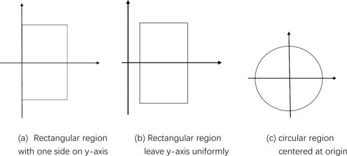
Three possible regions containing unstable roots
-
(ii)
If the estimate
$$ -\mu \bigl(KL^{-1}\bigr)-\frac{ \Vert L^{-1} \Vert \Vert M \Vert + \Vert K \Vert \Vert L^{-1} \Vert ^{2} \Vert N \Vert }{1- \Vert L ^{-1} \Vert \Vert N \Vert }>0 $$is true, one can find a positive number β satisfying
$$ -\mu \bigl(KL^{-1}\bigr)-\frac{ \Vert L^{-1} \Vert \Vert M \Vert + \Vert K \Vert \Vert L^{-1} \Vert ^{2} \Vert N \Vert }{1- \Vert L ^{-1} \Vert \Vert N \Vert }\max _{1\leq j\leq d}\bigl[e^{-\frac{\tau _{j}}{s}}\bigr]=\beta , $$and then the inequalities
$$ \beta \leq \operatorname{Re}(s)\leq \mu \bigl(-KL^{-1}\bigr)+ \frac{ \Vert L^{-1} \Vert \Vert M \Vert + \Vert K \Vert \Vert L^{-1} \Vert ^{2} \Vert N \Vert }{1- \Vert L^{-1} \Vert \Vert N \Vert }\max_{1\leq j\leq d}\bigl[e^{-\frac{ \beta \tau _{j}}{m^{2}}}\bigr], $$and
$$\begin{aligned}& -\mu \bigl(-iKL^{-1}\bigr)-\frac{ \Vert L^{-1} \Vert \Vert M \Vert + \Vert K \Vert \Vert L^{-1} \Vert ^{2} \Vert N \Vert }{1- \Vert L ^{-1} \Vert \Vert N \Vert }\max _{1\leq j\leq d}\bigl[e^{-\frac{\beta \tau _{j}}{m^{2}}}\bigr] \leq \operatorname{Im}(s) \\& \quad \leq \mu \bigl(iKL^{-1}\bigr)+\frac{ \Vert K^{-1} \Vert \Vert M \Vert + \Vert K \Vert \Vert L^{-1} \Vert ^{2} \Vert N \Vert }{1- \Vert L^{-1} \Vert \Vert N \Vert }\max _{1\leq j\leq d}\bigl[e^{-\frac{\beta \tau _{j}}{m^{2}}}\bigr] \end{aligned}$$are valid. Here
$$ m= \Vert K \Vert \bigl\Vert L^{-1} \bigr\Vert + \frac{ \Vert L^{-1} \Vert \Vert M \Vert + \Vert K \Vert \Vert L^{-1} \Vert ^{2} \Vert N \Vert }{1- \Vert L^{-1} \Vert \Vert N \Vert }. $$The inequalities mean that all possible unstable roots are located in a region strictly leaving the imaginary axis. See Fig. 1(b).

Proof
(i) As in Lemma 3.6, we have
Besides, the imaginary part of an eigenvalue of a matrix W is equivalent to the real part of an eigenvalue of \(-iW\), therefore,
From the left inequality above, we get
while from the right inequality, we get
Hence the second inequality holds.
(ii) By Lemma 3.3,
As in Lemma 3.6, we get
Let
Inequality (8) implies
where the last inequality can be derived from the following argument: set \(s=s_{1}+s_{2}i\) and \(s_{1}=\operatorname{Re}(s)>0\), then
where
Then
which means
Hence, taking (9) into consideration, we have
Let
Then we have
Let
Then we have
The iteration
and the monotonicity
assure that the limit of the sequence \(\{\beta _{j}\}\) is equal to β, where β is a positive number satisfying
Therefore the first inequality holds. Similarly, the second inequality can be obtained. □
We list two examples to illustrate two differential rectangular regions in Figs. 1(a) and 1(b). In Fig. 1(a), we can see Example 1 of Sect. 5. In that case, the rectangular region is
In Fig. 1(b), we try to create random matrices K, L and M from Matlab. Letting \(N=0\), we have
We compute:
here β is a positive solution of the equation, computation of \(\mu (*)\) refers to Theorem 5.1 in the last section. Also
Thus the rectangular region is
It is located on the right half-plane, which strictly leaves the imaginary axis.
As for systems of (1) in [8], we have a region including all the roots with nonnegative real parts when the condition of Corollary 3.1 fails.
Corollary 3.2
Let \(\|B^{-1}\|\cdot \|D\|<1\). Suppose that there exists a root of \((*)\) whose real part is nonnegative.
-
(i)
If we have the estimate
$$ \mu \bigl(-AB^{-1}\bigr)+\frac{ \Vert B^{-1} \Vert \Vert C \Vert + \Vert A \Vert \Vert B^{-1} \Vert ^{2} \Vert D \Vert }{1- \Vert B ^{-1} \Vert \Vert D \Vert }>0, $$then the inequalities
$$ 0\leq \operatorname{Re}(s)\leq \mu \bigl(-AB^{-1}\bigr)+ \frac{ \Vert B^{-1} \Vert \Vert C \Vert + \Vert A \Vert \Vert B ^{-1} \Vert ^{2} \Vert D \Vert }{1- \Vert B^{-1} \Vert \Vert D \Vert }, $$and
$$\begin{aligned} &{-}\mu \bigl(-iAB^{-1}\bigr)-\frac{ \Vert B^{-1} \Vert \Vert C \Vert + \Vert A \Vert \Vert B^{-1} \Vert ^{2} \Vert D \Vert }{1- \Vert B^{-1} \Vert \Vert D \Vert } \\ &\quad \leq \operatorname{Im}(s)\leq \mu \bigl(iAB^{-1}\bigr)+ \frac{ \Vert B^{-1} \Vert \Vert C \Vert + \Vert A \Vert \Vert B^{-1} \Vert ^{2} \Vert D \Vert }{1- \Vert B^{-1} \Vert \Vert D \Vert } \end{aligned}$$hold.
-
(ii)
If we have the estimate
$$ -\mu \bigl(AB^{-1}\bigr)-\frac{ \Vert B^{-1} \Vert \Vert C \Vert + \Vert A \Vert \Vert B^{-1} \Vert ^{2} \Vert D \Vert }{1- \Vert B ^{-1} \Vert \Vert D \Vert }>0 $$and define a positive number β by
$$ -\mu \bigl(AB^{-1}\bigr)-\frac{ \Vert B^{-1} \Vert \Vert C \Vert + \Vert A \Vert \Vert B^{-1} \Vert ^{2} \Vert D \Vert }{1- \Vert B ^{-1} \Vert \Vert D \Vert }\bigl[e^{-\frac{\tau _{j}}{m}} \bigr]=\beta , $$then the inequalities
$$ \beta \leq \operatorname{Re}(s)\leq \mu \bigl(-AB^{-1}\bigr)+ \frac{ \Vert B^{-1} \Vert \Vert C \Vert + \Vert A \Vert \Vert B^{-1} \Vert ^{2} \Vert D \Vert }{1- \Vert B^{-1} \Vert \Vert D \Vert }\bigl[e^{-\frac{\beta \tau _{j}}{m ^{2}}}\bigr], $$and
$$\begin{aligned}& -\mu \bigl(-iAB^{-1}\bigr)-\frac{ \Vert B^{-1} \Vert \Vert C \Vert + \Vert A \Vert \Vert B^{-1} \Vert ^{2} \Vert D \Vert }{1- \Vert B ^{-1} \Vert \Vert D \Vert }\bigl[e^{-\frac{\beta \tau _{j}}{m^{2}}} \bigr]\leq \operatorname{Im}(s) \\& \quad \leq \mu \bigl(iAB^{-1}\bigr)+\frac{ \Vert B^{-1} \Vert \Vert C \Vert + \Vert A \Vert \Vert B^{-1} \Vert ^{2} \Vert D \Vert }{1- \Vert B^{-1} \Vert \Vert D \Vert } \bigl[e^{-\frac{\beta \tau _{j}}{m^{2}}}\bigr] \end{aligned}$$are valid. Here
$$ m= \Vert A \Vert \bigl\Vert B^{-1} \bigr\Vert + \frac{ \Vert B^{-1} \Vert \Vert C \Vert + \Vert A \Vert \Vert B^{-1} \Vert ^{2} \Vert D \Vert }{1- \Vert B^{-1} \Vert \Vert D \Vert }. $$The inequalities imply that all possible unstable roots are located in a region strictly leaving the imaginary axis.
The following theorem denotes another kind of region which contains possible unstable roots. Different from Theorem 3.1, Theorem 3.2 gives an unstable region which is a circle centered at the origin. See Fig. 1(c).
Theorem 3.2
Let \(\|L^{-1}\|\cdot \|N\|<1\). If s is a characteristic root of (5) with nonnegative real part, then the inequality
holds.
Proof
By the assumption above, there exists an integer \(j (1\leq j\leq d)\) such that
This implies the inequality
It is obvious that
Therefore, due to Lemma 3.2, we obtain the claim. □
In accordance, we have this circle regions for system (1) in Corollary 3.3.
Corollary 3.3
Let \(\|B^{-1}\|\cdot \|D\|<1\). If s is a characteristic root of NDDAEs with nonnegative real part, then the inequality
is valid.
4 Boundary criteria for NDDAEs
In this section, we will give boundary criteria for delay dependent stability of system (2). Let
Applying Lemma 3.6, if \(\gamma <0\), system (2) is asymptotically stable. If \(\gamma \geq 0\), system (2) may be stable or unstable. We give stability criteria of (2) when \(\gamma \geq 0\). Let
and \(\gamma \geq 0\). We define the following quantities according to the sign of \(\beta _{0}\) (see Theorem 3.1):
(i) If \(\beta _{0}\leq 0\), we put
(ii) If \(\beta _{0}>0\), we put
where β is a root of the equation
Now we will list three kinds of bounded regions in the s-plane.
Definition 4.1
Let \(l_{1}\), \(l_{2}\), \(l_{3}\) and \(l_{4}\) denote the segments \(\{(E_{0}, y): F_{0}< y< F\}\), \(\{(x,F): E_{0}\leq x\leq E\}\), \(\{(E,y): F_{0}\leq y \leq F\}\), and \(\{(x, F_{0}): E_{0}\leq x \leq E\}\), respectively. Furthermore, let \(l=l_{1}\cup l_{2}\cup l_{3}\cup l_{4}\) and let D be the rectangular region surrounded by l.
Definition 4.2
Let \(R=\rho [(|K|+|M|)\cdot |L^{-1}|\cdot (I-|NL^{-1}|)^{-1}]\). Let \(\mathcal{K}\) denote the circular region with radius R centered at the origin of the plane of C:
Definition 4.3
Let T represent the intersection \(D\cap \mathcal{K}\). The boundary of T is denoted by ∂T and \(\overline{T}=T\cup \partial T\).
The following two theorems give criteria for the delay-dependent stability of system (2). Theorems 2.1 and 2.2, respectively, are crucial to prove them.
Theorem 4.1
If for any \((x,y)\in \partial T\), the real part \(\operatorname{Re}(x,y)\) in (6) is not equal to zero, then system (2) is asymptotically stable.
Proof
Suppose that the system (2) is unstable while the condition is not satisfied, then there exists a characteristic root of (5) whose real part is nonnegative. Using Lemma 3.1, one just needs to prove that \(P(s)\neq 0\) for \(\operatorname{Re}(s)\geq 0\). Applying Theorems 3.1 and 3.2 as well as Definition 4.3, it is sufficient to discuss the root \(s\in \overline{T}\). Recall the condition of this theorem and results of Theorem 2.1, together they obviously contradict \(P(s)=0\) when \(s\in \overline{T}\). Thus \(P(s)\neq 0\) for \(\operatorname{Re}(s)\geq 0\) and the proof is completed. □
The following Theorem 4.2 is a special case of Theorem 4.1.
Theorem 4.2
Assume that for any \((x,y)\in \partial T\), there exists a real constant λ satisfying
Then system (2) is asymptotically stable.
According to Definition 4.3, Theorems 4.1 and 4.2, if system (2) has unstable characteristic roots, they will be in an intersection part of a rectangle and a half-circle, both specified by the system.
5 Examples
In this section, we will give two examples to show the region which includes unstable characteristic roots of a system. Then we will apply backward differentiation formulae to the system and check the analytical stability by numerical behavior. The following theorem gives a way to find the logarithmic norms of a matrix.
Theorem 5.1
([13])
Let \(x=(x_{1}, x_{2}, \ldots , x_{n})^{T}\in \mathbb{C}^{n}\), \(W=(\omega _{ij})\in \mathbb{C}^{n\times n}\), then
Here \(W^{*}\) denotes the complex conjugate transpose of matrix W. It can be seen that \(\mu (W)\) is easy to compute in cases \(p=1, 2, \infty \). It can also be seen that \(\mu (W)\) may actually be smaller than the corresponding \(\|W\|\), or \(\mu (W)\) may even be negative.
In the following Example 1, we choose same delay in different components, while in Example 2, we take different delays for corresponding components. We find that the two situations produce different phenomena. Therefore, delay-dependent stability has more information than delay-independent stability.
Example 1
Consider the following strangeness-free NDDAEs:
where
\(\tau _{1}=\tau _{2}=\tau _{3}=1\), and \(\phi (t)= (\cos t, \sin t, \cos 3t )^{T}\). As in Corollary 3.3, let
By virtue of Lemma 3.6, if \(\gamma <0\), system (2) is asymptotically stable. If \(\gamma \geq 0\), system (2) may be stable or unstable. We consider the stability of (2) when \(\gamma \geq 0\). Let
and \(\gamma \geq 0\). We define the following quantities according to the sign of \(\beta _{0}\).
We find that:
Solving \(P(s)=0\), we get \(s=-1.99699\). Thus conditions of Theorem 4.1 are satisfied and the system is asymptotically stable. We could check its stability by applying BDF methods to the system with step size \(h=0.1\). Three components and 2-norm value of the solution vector are listed in the four graphs of Fig. 2.

Numerical solutions of three components for Example 1
Example 2
We study the same system as in Example 1 but choose different delays, that is, \(\tau _{1}=1\), \(\tau _{2}=2\), \(\tau _{3}=3\). Then, although the system is also stable, we can see from Fig. 3 that stability of the system with different delays on corresponding component has larger fluctuation than for the system with same delay in each component. So for a generalized neutral system, delay-dependent stability analysis has more information and is more useful than delay-independent stability analysis.

Numerical solutions of three components for Example 2
Therefore, we have given two criteria for the delay-dependent stability of the linear delay system (2). Theorems 3.1 and 3.2 show that the unstable characteristic roots of system (2) are located in some specified bounded region in the complex plane, while Theorems 4.1 and 4.2 show that it is sufficient to check certain conditions on its boundary to exclude the possibility of such roots from the region.
References
Hu, G., Mitsui, T.: Stability of linear systems with matrices having common eigenvectors. Jpn. J. Ind. Appl. Math. 13, 487–494 (1996)
Lin, Q., Kuang, J.X.: On the LD-stability of the nonlinear systems in MDBMs. J. Shanghai Teach. Univ. Nat. Sci. 25(4) (1996)
Kuang, J., Cong, Y.: Stability of Numerical Methods for Delay Differential Equations. Science Press, Beijing (2005)
Sun, L.: Stability analysis for delay differential equations with multidelays and numerical examples. Math. Comput. 75(253), 151–165 (2005)
Sun, L.: Asymptotic stability for the system of neutral delay differential equations. Appl. Math. Comput. 218, 337–345 (2011)
Hu, G.-D.: Computable stability criterion of linear neutral systems with unstable difference operators. J. Comput. Appl. Math. 271, 223–232 (2014)
Ascher, U., Petzold, L.R.: The numerical solution of delay-differential-algebraic equations of retarded and neutral type. SIAM J. Numer. Anal. 32, 1635–1657 (1995)
Zhu, W., Petzold, L.R.: Asymptotic stability of linear delay differential-algebraic equations and numerical methods. Appl. Numer. Math. 24, 247–264 (1997)
Campbell, S.L., Linh, V.H.: Stability criteria for differential-algebraic equations with multiple delays and their numerical solutions. Appl. Math. Comput. 208, 397–415 (2009)
Michiels, W.: Spectrum-based stability analysis and stabilisation of systems described by delay differential-algebraic equations. IET Control Theory Appl. 5, 1829–1842 (2011)
Biegler, L.T., Campbell, S.L., Mehrmann, V.: Control and Optimaization with Differential-Algebraic Constraints. SIAM, Philadelphia (2012)
IIchmann, A., Reis, T.: Surveys in Differential-Algebraic Equations I. Springer, Berlin (2013)
Du, N.H., Linh, V.H., Mehrmann, V., Thuan, D.D.: Stability and robust stability of linear time-invariant delay differential-algebraic equations. SIAM J. Matrix Anal. Appl. 34, 1631–1654 (2013)
Lamour, R., Marz, R., Tischendorf, C.: Differential-Algebraic Equations: A Projector Based Analysis. Springer, Berlin (2013)
IIchmann, A., Reis, T.: Surveys in Differential-Algebraic Equations II. Springer, Cham (2015)
IIchmann, A., Reis, T.: Surveys in Differential-Algebraic Equations III. Springer, Cham (2015)
Betts, J.T., Campbell, S.L., Thompson, K.: Solving optimal control problems with control delays using direct transcription. Appl. Numer. Math. 108, 185–203 (2016)
Campbell, S.L., Kunkel, P.: Solving higher index DAE optimal control problems. Numer. Algebra Control Optim. 6, 447–472 (2017)
Liao, H., Sun, L., Huang, Z.: A new stability analysis for a class of nonlinear delay differential-algebraic equations and implicit Euler methods. J. Shanghai Norm. Univ. Nat. Sci. 47(4) (2018)
Ha, P.: Spectral characterizations of solvability and stability for delay differential-algebraic equations. Acta Math. Vietnam. 43(4), 715–735 (2018)
Golub, G., Van Loan, C.F.: Matrix Computations, 3rd edn. Johns Hopkins University Press, Baltimore (1996)
Desoer, C.A., Vidyasagar, M.: Feedback System: Input–Output Properties. Academic Press, New York (1997)
Acknowledgements
The research is supported by the Scientific Computing Key Laboratory of Shanghai University and the Shanghai Natural Science Foundation, No. 15ZR1431200.
Availability of data and materials
Not applicable.
Funding
Not applicable.
Author information
Authors and Affiliations
Contributions
The entire paper is finished by one author. The author read and approved the final manuscript.
Corresponding author
Ethics declarations
Competing interests
The author declares that he has no competing interests.
Additional information
Publisher’s Note
Springer Nature remains neutral with regard to jurisdictional claims in published maps and institutional affiliations.
Rights and permissions
Open Access This article is distributed under the terms of the Creative Commons Attribution 4.0 International License (http://creativecommons.org/licenses/by/4.0/), which permits unrestricted use, distribution, and reproduction in any medium, provided you give appropriate credit to the original author(s) and the source, provide a link to the Creative Commons license, and indicate if changes were made.
About this article

Cite this article
Sun, L. Stability criteria for neutral delay differential-algebraic equations with many delays. Adv Differ Equ 2019, 343 (2019). https://doi.org/10.1186/s13662-019-2265-3
Received:
Accepted:
Published:
DOI: https://doi.org/10.1186/s13662-019-2265-3