Modeling plant virus propagation with Filippov control

Abstract

Plants play a vital role in the everyday life of all organisms on earth. This paper proposes a Filippov vector-borne plant disease model incorporating roguing of infected plants and spaying pesticides to relieve the economical devastation for growers and damage to humans, natural enemies and the environment. No control strategy is taken if the number of infected plants is less than an infected plant threshold level $I_{c}$; further, infected plants are removed once the number of infected plants exceeds $I_{c}$; meanwhile, pesticides are spayed if the number of infected vectors exceeds the infected vector threshold level $Y_{c}$. The global dynamics for the proposed system is investigated. Model solutions ultimately stabilize at the positive equilibrium that lies in the region above $I_{c}$, or on $I=I_{c}$, or below $I_{c}$, depending on the threshold values $I_{c}$ and $Y_{c}$. The findings indicate that proper combinations of the infected plant and vector threshold values based on the threshold policy can maintain the number of infected plants either at a previously given level or below a certain threshold level.

1 Introduction

Plant viruses belong to the most limiting factors to modern agriculture, especially in lesser-developed countries. For example, the cassava mosaic virus has ravaged the cassava plant, a staple in many underdeveloped African countries, in Kenya, Uganda and Tanzania [1]. Tomato in India is another example of plants infected by viruses. These viruses cause tomato leaf curling disease (TLCD), such that diseased plants exhibit vein clearing, leaf curling, stunting and partial or complete sterility [1, 2]. Most plant viruses are vectored by arthropods, notably homopteran insects [1]. In fact, insects are responsible for 70% of all plant virus transmissions [3]. The vector that transmits both the cassava mosaic virus and TLCD is Bemisia tabaci.

Roguing (identifying and removal of diseased plants) is a well-known means of virus disease control measures with wide applicability [1]. It has been recommended repeatedly to control cassava mosaic disease. However, roguing is generally unpopular with farmers, who will suffer crop loss and are short of energy to allocate effort and time required to inspect crops with the thoroughness and frequency required to identify and remove diseased plants [4, 5]. Vector control by using pesticides (insecticides, acaricides, nematicides and fungicides) against the insect or mite vectors [4] has been used successfully to prevent or at least decrease the transmission of the virus. However, the use of chemicals is not always applicable or appropriate, one disadvantage being the damage to natural enemies and risks to human health and the environment [4].

Mathematical modeling has increasingly been developed using a wide range of techniques and used to the study of plant virus disease epidemics [6–14]. Gao et al. [15] used a model to evaluate the effects of control measures when roguing and replanting were practiced. The authors showed that previous models that modeled roguing as a continuous activity may over estimate the infection risk compared with the more realistic intermittent roguing. van den Bosch and Jeger [16] adapted the model proposed in Ref [17] to evaluate the effect of control interventions on cassava mosaic disease dynamics. The results showed that a combination of disease management measures including both continuous roguing and spaying insecticide might eradicate the disease.

Since completely removal of diseased plants is generally unachievable, nor is it economically or biologically desirable, then control measures should be implemented such that the number of diseased plants stabilize at a desired or an acceptable level (the economic threshold in IDM–integrated disease management [11]). IDM allows an economic threshold, a tolerant threshold beyond which control measures are implemented to prevent the number of infected plants from exceeding the acceptable level. Accordingly, Filippov systems modeled by using nonlinear differential equations with discontinuous right-hand sides are proposed by incorporating these control strategies to investigate the transmission of plant disease. The authors in Refs [18, 19] established and investigated the Filippov-type models by considering a proportional planting rate and a constant planting rate, respectively. The effectiveness of the control measures was evaluated to maintain the number of diseased plants not exceeding the economic threshold.

In order to relieve the economical devastate for growers by continuously roguing diseased plants and the damage to the environment, human health and natural enemies by spraying insecticides, in this paper, we consider a vector-borne plant disease model with Filippov–type control, that is, roguing and spraying insecticides are implemented only when the infected plants and infected vectors are beyond some tolerant thresholds. The Filippov vector-borne plant disease model is proposed in Sect. 2. The existence and global stability of various types of positive equilibria and the existence of the sliding mode and its dynamics are investigated by varying the infected plant and vector threshold values in Sects. 3–6. A conclusion together with biological implications is presented in Sect. 7.

2 Filippov vector-borne plant disease model

We consider a threshold policy to control the transmission of the plant disease and achieve the maximal economic benefits with roguing diseased plants and spaying insecticides. Here the numbers of infected plants and vectors are chosen as two indices to decide on when to take control strategies. The threshold policy is defined as follows: we take no control strategy when the number of infected plants is less than the infected plant threshold level $I_{c}$; we remove diseased plants at a rate q once the number of infected plants exceeds $I_{c}$; meanwhile we spray insecticides if the number of infected vectors exceeds the infected vector threshold value $Y_{c}$; whereas we only remove diseased plants at a rate q if the infected vectors are less than $Y_{c}$, which seems realistic from the point of view of relieving the damage of insecticides to environment, human health and natural enemies. A schematic diagram of the threshold policy is illustrated in Fig. 1.

Figure 1

Schematic diagram of the threshold policy

Plant population is divided into susceptible plants S and infected plants I. Susceptible plants do not have the disease but can contract the disease if infected with the virus. The infected plants have the virus but cannot directly transmit the virus to susceptible plants. Infected plants can either die from the disease or recover. We assume that, as soon as a plant dies either from the infection or from a natural death, it is immediately replaced with a new susceptible plant by a grower. Thus the total plant population $K=S+I$ remains fixed.

The insect vector population is divided into susceptible insect vectors X and infected insect vectors Y. The susceptible insects do not have the virus but can obtain the virus if they come in contact with an infected plant. Infected insects can transmit the virus to susceptible plants upon contact. We assume no vertical transmission of the virus with neither vectors nor plants. Moreover, we assume that the virus does not harm the vector and it holds the virus for the rest of its life. We consider a bilinear incidence rate, then the model describing the interactions of the plants and the vectors reads as follows:

$$\begin{aligned}& \frac{dX}{dt}=\varLambda -\beta _{1}XI-mX, \\& \frac{dY}{dt}=\beta _{1}XI-mY, \\& \frac{dS}{dt}=\mu K+(d+\gamma )I-\mu S-\beta _{p}SY, \\& \frac{dI}{dt}=\beta _{p}SY-(d+\mu +\gamma )I, \end{aligned}$$

where Λ is the replenishing rate of vectors (birth and/or immigration), m (μ) is the natural death rate of vectors (plants), $\beta _{1}$ ($\beta _{p}$) is the infection rate of vectors (plants) due to plants (vectors), d is the disease deduced death rate of infected plants, γ is the recovery rate of plants. Notice that adding $\frac{dX}{dt}$ and $\frac{dY}{dt}$ yields

$$ \frac{dN}{dt}=\varLambda -mN, $$

where $N=X+Y$ and as $t\rightarrow \infty$, $N\rightarrow \frac{\varLambda }{m}$.

So we can consider a reduced system with the threshold policy depicted in Fig. 1 as follows:

$$ \begin{pmatrix} Y^{\prime } \\ I^{\prime } \end{pmatrix}=f(Y,I)= \begin{pmatrix} \beta _{1} I (\frac{\varLambda }{m}-Y )-mY-u_{1}Y \\ \beta _{p} Y(K-I)-\omega I-u_{2}I \end{pmatrix}, $$

(1)

with

$$ (u_{1}, u_{2})= \textstyle\begin{cases} (0,0), & \text{for } I< I_{c}, \\ (0,q), & \text{for } Y< Y_{c} \text{ and } I>I_{c}, \\ (v, q), & \text{for } Y>Y_{c} \text{ and } I>I_{c}, \end{cases} $$

(2)

where $\omega =d+\mu +\gamma$, q is the roguing rate, and v is the insecticide spray induced death rate of vectors.

Therefore, the Y, I space $R_{+}^{2}$ can be divided into the following five regions:

$$\begin{aligned}& G_{1}= \bigl\{ (Y,I)\in R_{+}^{2}: I< I_{c} \bigr\} , \\& G_{2}= \bigl\{ (Y,I)\in R_{+}^{2}: Y< Y_{c} \text{ and } I>I_{c} \bigr\} , \\& G_{3}= \bigl\{ (Y,I)\in R_{+}^{2}: Y>Y_{c} \text{ and } I>I_{c} \bigr\} , \\& \varOmega _{1}= \bigl\{ (Y,I)\in R_{+}^{2}: I=I_{c} \bigr\} , \\& \varOmega _{2}= \bigl\{ (Y,I)\in R_{+}^{2}: Y=Y_{c} \text{ and } I>I_{c} \bigr\} . \end{aligned}$$

The dynamics in region $G_{i}$ are governed by $F_{i}$, for $i=1,2,3$, where

$$\begin{aligned}& F_{1}(Y,I)= \begin{pmatrix} F_{11}(Y,I) \\ F_{12}(Y,I) \end{pmatrix}= \begin{pmatrix} \beta _{1} I (\frac{\varLambda }{m}-Y )-mY \\ \beta _{p} Y(K-I)-\omega I \end{pmatrix}, \end{aligned}$$

(3)

$$\begin{aligned}& F_{2}(Y,I)= \begin{pmatrix} F_{21}(Y,I) \\ F_{22}(Y,I) \end{pmatrix}= \begin{pmatrix} \beta _{1} I (\frac{\varLambda }{m}-Y )-mY \\ \beta _{p} Y(K-I)-\omega I-qI \end{pmatrix}, \end{aligned}$$

(4)

$$\begin{aligned}& F_{3}(Y,I)= \begin{pmatrix} F_{31}(Y,I) \\ F_{32}(Y,I) \end{pmatrix}= \begin{pmatrix} \beta _{1} I (\frac{\varLambda }{m}-Y )-mY-vY \\ \beta _{p} Y(K-I)-\omega I-qI \end{pmatrix}. \end{aligned}$$

(5)

Note that the manifolds $\varOmega _{1}$ and $\varOmega _{2}$ are discontinuity surfaces between the two different structures of system (1) with (2). The normal vectors that are perpendicular to $\varOmega _{1}$ and $\varOmega _{2}$ are defined as $n_{1} = (0, 1)^{T}$ and $n_{2} = (1, 0)^{T}$, respectively. The existence and uniqueness of solutions of Filippov system, such as system (1) with (2), is illustrated elaborately in Ref [20]. Here, we just present some definitions (real and/or virtual equilibrium, pseudoequilibrium, sliding modes) that will be used in what follows, detailed contents can be referred to [20–23].

Definition 2.1

A point $E^{*}$ is called a real equilibrium of system (1) with (2) if $F_{i}(E^{*})=0$, and $E^{*}\in G_{i}$, $i=1, 2, 3$; $E^{*}$ is called a virtual equilibrium if $F_{i}(E^{*})=0$, and $E^{*}\in G_{j}$, $j\neq i$, $i, j=1, 2, 3$.

Definition 2.2

A point $E^{P}$ is called a pseudoequilibrium of system (1) with (2) if it is an equilibrium of the sliding mode of system (1) with (2). A sliding mode exists if there are subsets Σ of the manifold $\varOmega _{i}$ such that the flows of f (outside of $\varOmega _{i}$) are directed toward each other on them, $i=1,2$.

Definition 2.3

The set of all points $(Y,I)$ on $\varOmega _{j}$ such that the flow of f (outside $\varOmega _{j}$) approaches $(Y,I)$ from all sides is an attracting sliding mode, $j=1,2$. When the attraction sliding mode is only one point, it is said to be a pseudoattractor.

2.1 Dynamics of the subsystems $F_{i}$ in region $G_{i}$, $i=1,2,3$

In this section, we investigate the global dynamics of $F_{i}$ in region $G_{i}$, $i=1,2,3$. The basic reproduction number $R_{0i}$ (the average number of secondary cases of an infectious disease arising from a typical case in a totally susceptible population) for the system in region $G_{i}$, $i=1,2,3$, can be defined by applying the next generation matrix method [24], where

$$ R_{01}=\frac{K \varLambda \beta _{1}\beta _{p}}{m^{2}\omega },\quad\quad R_{02}= \frac{K \varLambda \beta _{1}\beta _{p}}{m^{2}(\omega +q)}, \quad\quad R_{03}= \frac{K \varLambda \beta _{1}\beta _{p}}{m(m+v)(\omega +q)}. $$

The system in region $G_{i}$ always has one disease-free equilibrium given by $E_{i0}$, $i=1,2,3$. Furthermore, if $R_{0i}>1$, there is a unique endemic equilibrium given by $E_{i}=(Y_{i}^{*}, I_{i}^{*})$, where

$$\begin{aligned}& E_{10}=(0,0), \quad\quad E_{1}=\bigl(Y_{1}^{*}, I_{1}^{*}\bigr)= \biggl( \frac{\beta _{1}\frac{\varLambda }{m}I_{1}^{*}}{\beta _{1}I_{1}^{*}+m}, \frac{K\beta _{1}\beta _{p}\frac{\varLambda }{m}-m\omega }{\beta _{1}\beta _{p}\frac{\varLambda }{m}+\beta _{1}\omega } \biggr), \\& E_{20}=(0,0), \quad\quad E_{2}=\bigl(Y_{2}^{*}, I_{2}^{*}\bigr)= \biggl( \frac{\beta _{1}\frac{\varLambda }{m}I_{2}^{*}}{\beta _{1}I_{2}^{*}+m}, \frac{K\beta _{1}\beta _{p}\frac{\varLambda }{m}-m(\omega +q)}{\beta _{1}\beta _{p}\frac{\varLambda }{m}+\beta _{1}(\omega +q)} \biggr), \\& E_{30}=(0,0), \quad\quad E_{3}=\bigl(Y_{3}^{*}, I_{3}^{*}\bigr)= \biggl( \frac{\beta _{1}\frac{\varLambda }{m}I_{3}^{*}}{\beta _{1}I_{3}^{*}+m+v}, \frac{K\beta _{1}\beta _{p}\frac{\varLambda }{m}-(m+v)(\omega +q)}{\beta _{1}\beta _{p}\frac{\varLambda }{m}+\beta _{1}(\omega +q)} \biggr). \end{aligned}$$

The following proposition gives the global stability of the equilibria in region $G_{i}$, $i=1,2,3$.

Proposition 2.1

(i) If $R_{0i}<1$, then the disease-free equilibrium $E_{i0}$is globally asymptotically stable; (ii) If $R_{0i}>1$, then the endemic equilibrium $E_{i}$is globally asymptotically stable, $i=1,2,3$.

Proof

The corresponding Jacobian matrix of system (1) with (2) equals

$$ J= \begin{pmatrix} -\beta _{1}I-m-u_{1} & \beta _{1}\frac{\varLambda }{m} \\ \beta _{p}(K-I) & -\beta _{p}Y-\omega -u_{2} \end{pmatrix}. $$

(i) At $E_{i0}$ in region $G_{i}$,

$$ \begin{gathered} p=-\operatorname{tr} J=m+\omega +u_{1}+u_{2}, \\ q= \vert J \vert =(m+u_{1}) (\omega +u_{2}) (1-R_{0i}). \end{gathered} $$

Hence, if $R_{0i}<1$ the characteristic equation has two negative eigenvalues, $E_{i0}$ is locally asymptotically stable. Further, choosing a Dulac function $B=1/(YI)$, we have

$$ \frac{\partial (BF_{i1})}{\partial Y}+ \frac{\partial (BF_{i2})}{\partial I}=- \biggl( \frac{\beta _{1}\frac{\varLambda }{m}}{Y^{2}}+ \frac{K\beta _{p}}{I^{2}} \biggr) < 0, \quad i=1,2,3. $$

Thus by the Bendixson–Dulac criterion, $E_{i0}$ is globally asymptotically stable by excluding the existence of limit cycles, $i=1,2,3$.

(ii) If $R_{0i}>1$,

$$ \begin{gathered} p=-\operatorname{tr}J=\beta _{1}I_{i}^{*}+m+ \beta _{p}Y_{i}^{*}+\omega +u_{1}+u_{2}, \\ q= \vert J \vert =\beta _{1}\beta _{p}Y_{i}^{*}I_{i}^{*}+ \beta _{p}Y_{i}^{*}(m+u_{1}). \end{gathered} $$

So $E_{i}$ is locally asymptotically stable for there exists two negative eigenvalues. Similarly, $E_{i}$ is globally asymptotically stable, $i=1,2,3$, by the Bendixson–Dulac criterion with the Dulac function $B=1/(YI)$. □

2.2 Sliding mode on $\varOmega _{1}$ and its dynamics

Note that a sliding surface may exist on $\varOmega _{1}$ between the regions $G_{1}$ and $G_{2}$, or between the regions $G_{1}$ and $G_{3}$. First, from $\langle n_{1}, F_{1}\rangle > 0$, we have $Y>\frac{\omega I_{c}}{\beta _{p}(K-I_{c})}\doteq h_{1}$, and from $\langle n_{1}, F_{2}\rangle <0$, we have $Y<\frac{(\omega +q) I_{c}}{\beta _{p}(K-I_{c})}\doteq h_{2}$, hence, there may exist a sliding mode on $\varOmega _{1}$ between the regions $G_{1}$ and $G_{2}$, which is defined as

$$ \varSigma _{1}=\bigl\{ (Y, I) \in \varOmega _{1}: h_{1}< Y< \min \{h_{2},Y_{c}\} \bigr\} . $$

(6)

Then we investigate the dynamics on $\varSigma _{1}\subset \varOmega _{1}$. Utilizing the Filippov convex method [25, 26], we have

$$ \begin{pmatrix} Y^{\prime } \\ I^{\prime } \end{pmatrix}=\sigma _{1}F_{1}+(1-\sigma _{1})F_{2}, \quad \text{where } \sigma _{1}= \frac{\langle n_{1}, F_{2}\rangle }{\langle n_{1}, F_{2}-F_{1}\rangle }. $$

Therefore, the sliding-mode dynamics along the manifold $\varSigma _{1}$ can be described by

$$ \textstyle\begin{cases} Y^{\prime }=\beta _{1} (\frac{\varLambda }{m}-Y )I_{c}-mY, \\ I^{\prime }=0. \end{cases} $$

(7)

System (7) exists a unique equilibrium $E_{p1}=(Y_{p1}^{*}, I_{c})$, where $Y_{p1}^{*}= \frac{\beta _{1}\frac{\varLambda }{m}I_{c}}{\beta _{1}I_{c}+m}$.

Next, from $\langle n_{1}, F_{1} \rangle >0$ and $\langle n_{1}, F_{3} \rangle <0$, there may also exist a sliding mode on $\varOmega _{1}$ between the regions $G_{1}$ and $G_{3}$, which is defined as

$$ \varSigma _{2}=\bigl\{ (Y, I) \in \varOmega _{1}: \max \{Y_{c}, h_{1}\}< Y< h_{2} \bigr\} . $$

(8)

Moreover, the sliding-mode dynamics along the manifold $\varSigma _{2}$ can be obtained by the Filippov convex method,

$$ \begin{pmatrix} Y^{\prime } \\ I^{\prime } \end{pmatrix}=\sigma _{2}F_{1}+(1-\sigma _{2})F_{3}, \quad \text{where } \sigma _{2}= \frac{\langle n_{1}, F_{3}\rangle }{\langle n_{1}, F_{3}-F_{1}\rangle }. $$

That is,

$$ \textstyle\begin{cases} Y^{\prime }=\beta _{1} (\frac{\varLambda }{m}-Y )I_{c}-mY- \frac{\beta _{p}Y(K-I_{c})-\omega I_{c}}{qI_{c}}vY, \\ I^{\prime }=0. \end{cases} $$

(9)

For system (9) there exists a unique equilibrium $E_{p2}=(Y_{p2}^{*}, I_{c})$, where $Y_{p2}^{*}=\frac{-b_{1}+\sqrt{b_{1}^{2}-4a_{1}c_{1}}}{2a_{1}}$,

$$ a_{1}=\beta _{p}(K-I_{c})v,\quad\quad b_{1}=(m+ \beta _{1}I_{c})qI_{c}-\omega vI_{c},\quad\quad c_{1}=- \beta _{1}\frac{\varLambda }{m}qI_{c}^{2}. $$

Finally, we present the conditions for different sliding modes $\varSigma _{1}$ and $\varSigma _{2}$ and seek conditions under which $E_{p1}$ and $E_{p2}$ become pseudoequilibria on $\varSigma _{1}\subset \varOmega _{1}$ and $\varSigma _{2}\subset \varOmega _{1}$. For convenience, we give the following notations that will be used throughout the analysis:

$$ \begin{gathered} g_{1} = \frac{mY_{c}}{\beta _{1}(\frac{\varLambda }{m}-Y_{c})}, \\ g_{2} = \frac{(m+v)Y_{c}}{\beta _{1}(\frac{\varLambda }{m}-Y_{c})}, \\ g_{3} = \frac{-b_{2}+\sqrt{b_{2}^{2}-4a_{2}c_{2}}}{2a_{2}}, \\ \quad \text{where } a_{2}=\beta _{1}q \biggl( \frac{\varLambda }{m}-Y_{c} \biggr), b_{2}=\beta _{p}vY_{c}^{2}-mqY_{c}+ \omega vY_{c}, c_{2}=-K\beta _{p}vY_{c}^{2}, \\ g_{4} = \frac{K\beta _{p}Y_{c}}{\omega +q+\beta _{p}Y_{c}}, \\ g_{5} = \frac{K\beta _{p}Y_{c}}{\omega +\beta _{p}Y_{c}}. \end{gathered} $$

(10)

Proposition 2.2

According to the value of $Y_{c}$, we have the following three situations.

• (1) If $Y_{c}< h_{1}$ ($I_{c}>g_{5}$by Proposition 2.3), then $\varSigma _{1}$does not exist, while $\varSigma _{2}=\{(Y,I)\in \varOmega _{1}: h_{1}< Y< h_{2}\}$.

  $E_{p1}$does not exist, while $E_{p2}\in \varSigma _{2}\subset \varOmega _{1}$if $h_{1}< Y_{p2}^{*}< h_{2}$, that is, if and only if $I_{3}^{*}< I_{c}< I_{1}^{*}$.

• (2) If $h_{1}< Y_{c}< h_{2}$ ($g_{4}< I_{c}< g_{5}$), then $\varSigma _{1}=\{(Y,I)\in \varOmega _{1}: h_{1}< Y< Y_{c}\}$, $\varSigma _{2}=\{(Y,I)\in \varOmega _{1}: Y_{c}< Y< h_{2}\}$.

  $E_{p1}\in \varSigma _{1}\subset \varOmega _{1}$if $h_{1}< Y_{p1}^{*}< Y_{c}$, that is, if and only if $I_{2}^{*}< I_{c}<\min \{I_{1}^{*}, g_{1}\}$;

  $E_{p2}\in \varSigma _{2}\subset \varOmega _{1}$if $Y_{c}< Y_{p2}^{*}< h_{2}$, that is, if and only if $\max \{I_{3}^{*},g_{3}\}< I_{c}< I_{1}^{*}$, where $g_{1}< g_{3}$if and only if $Y_{c}< Y_{1}^{*}$.

• (3) If $h_{2} < Y_{c}$ ($I_{c}< g_{4}$), then $\varSigma _{1}=\{(Y,I)\in \varOmega _{1}: h_{1}< Y< h_{2}\}$, while the sliding mode $\varSigma _{2}$does not exist.

  $E_{p1}\in \varSigma _{1}\subset \varOmega _{1}$if $h_{1}< Y_{p1}^{*}< h_{2}$, that is, if and only if $I_{2}^{*}< I_{c}< I_{1}^{*}$, while $E_{p2}$does not exist.

  The different sliding modes $\varSigma _{1}$and $\varSigma _{2}$on $\varOmega _{1}$according to the relationship between $g_{4}$, $g_{5}$and $I_{c}$are depicted in Fig. 2.

  Figure 2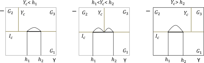

  

  Different sliding modes on $\varOmega _{1}$ according to the relationship between $g_{4}$, $g_{5}$ and $I_{c}$. The sliding-mode dynamics on $\varSigma _{1}$ can be described by Eq. (7), while the sliding-mode dynamics on $\varSigma _{2}$ can be described by Eq. (9). $h_{1}=\frac{\omega I_{c}}{\beta _{p}(K-I_{c})}$, $h_{2}= \frac{(\omega +q) I_{c}}{\beta _{p}(K-I_{c})}$

Proof

Here we present the derivation for $g_{3}$, other results can be obtained by lengthy but trivial calculation. In this case, $h_{1}< Y_{c}< h_{2}$, $E_{p2}$ becomes a pseudoequilibrium if $Y_{c}< Y_{p2}^{*}< h_{2}$. First we have $Y_{p2}^{*}< h_{2}$ if and only if $I_{c}>I_{3}^{*}$, $Y_{p2}^{*}>h_{1}$ if and only if $I_{c}< I_{1}^{*}$. Then we consider the situation when $Y_{c}< Y_{p2}^{*}$. By calculation, we obtain

$$ Y_{p2}^{*}-Y_{c}>0\quad \Longleftrightarrow\quad a_{2}I_{c}^{2}+b_{2}I_{c}+c_{2}>0, $$

where $a_{2}$, $b_{2}$ and $c_{2}$ are shown in Eq. (10). For $a_{2}>0$, $c_{2}<0$, we have $a_{2}I_{c}^{2}+b_{2}I_{c}+c_{2}>0 \Leftrightarrow I_{c}> \frac{-b_{2}+\sqrt{b_{2}^{2}-4a_{2}c_{2}}}{2a_{2}}=g_{3}$, where $g_{3}$ is the unique positive root of $a_{2}I_{c}^{2}+b_{2}I_{c}+c_{2}=0$. Then we have $Y_{p2}^{*}>Y_{c}\Leftrightarrow I_{c}>g_{3}$. By lengthy calculation we can also obtain $g_{1}< g_{3}\Leftrightarrow Y_{c}< Y_{1}^{*}$. □

The following theorems show the stability of $E_{p1}$ and $E_{p2}$.

Theorem 2.1

$E_{p1}$is stable on $\varSigma _{1}\subset \varOmega _{1}$when it is feasible.

Proof

We have

$$ \frac{\partial }{\partial Y} \biggl(\beta _{1} \biggl(\frac{\varLambda }{m}-Y \biggr)I_{c}-mY \biggr) \bigg| _{E_{p1}}=-\beta _{1}I_{c}-m< 0. $$

Hence, $E_{p1}$ is attracting. □

Note that the term “feasible” here means the equilibrium is a pseudoequilibrium throughout this paper.

Theorem 2.2

$E_{p2}$is stable on $\varSigma _{2}\subset \varOmega _{1}$when it is feasible.

Proof

We have

$$ \begin{gathered} \frac{\partial }{\partial Y} \biggl(\beta _{1} \biggl( \frac{\varLambda }{m}-Y \biggr)I_{c}-mY-\frac{\beta _{p}Y(K-I_{c})-\omega I_{c}}{qI_{c}}vY \biggr) \bigg| _{E_{p2}} \\ \quad =-\beta _{1}I_{c}- \frac{\beta _{p}(K-I_{c})}{qI_{c}}vY_{p2}^{*}- \beta _{1} \biggl( \frac{\varLambda }{m}-Y_{p2}^{*} \biggr)\frac{I_{c}}{Y_{p2}^{*}}< 0. \end{gathered} $$

Hence, $E_{p2}$ is attracting. □

Note that according to Proposition 2.2, the existence of the sliding modes $\varSigma _{1}$ and $\varSigma _{2}$ and the conditions under which $E_{p1}$ and $E_{p2}$ become pseudoequilibria on $\varSigma _{1}\subset \varOmega _{1}$ and $\varSigma _{2}\subset \varOmega _{1}$ depend on the relationship between the threshold value $Y_{c}$, $h_{1}$ and $h_{2}$. The next proposition gives the equivalent formula related to $I_{c}$.

Proposition 2.3

The following equivalent formula holds between $Y_{c}$and $I_{c}$:

$$\begin{aligned}& Y_{c}< h_{1} \quad \textit{if and only if} \quad I_{c}>g_{5}, \\& h_{1}< Y_{c} < h_{2} \quad \textit{if and only if} \quad g_{4}< I_{c}< g_{5}, \\& h_{2}< Y_{c} \quad \textit{if and only if} \quad I_{c}< g_{4}, \end{aligned}$$

where $g_{4}$and $g_{5}$are shown in Eq. (10).

Proposition 2.2 together with Proposition 2.3 can give the conditions for the existence of the sliding modes $\varSigma _{1}$ and $\varSigma _{2}$, and $E_{p1}$ and $E_{p2}$ to be pseudoequilibria related to $I_{c}$, $g_{4}$ and $g_{5}$.

2.3 Sliding mode on $\varOmega _{2}$ and its dynamics

A sliding surface may exist on $\varOmega _{2}$ between the regions $G_{2}$ and $G_{3}$. From $\langle n_{2}, F_{2}\rangle >0$, we have $I>\frac{mY_{c}}{\beta _{1}(\frac{\varLambda }{m}-Y_{c})} = g_{1}$. From $\langle n_{2}, F_{3}\rangle <0$, we have $I<\frac{(m+v)Y_{c}}{\beta _{1}(\frac{\varLambda }{m}-Y_{c})} = g_{2}$. Therefore, the sliding mode on $\varOmega _{2}$ is

$$ \varSigma _{3}=\bigl\{ (Y,I)\in \varOmega _{2}: \max \{I_{c},g_{1}\}< I< g_{2}, g_{2}>I_{c} \bigr\} . $$

(11)

Note that the relationship between $I_{c}$ and $g_{2}$ may be a little hard to be determined in some situations, so the sliding mode $\varSigma _{3}\subset \varOmega _{2}$ varies from one case to another.

Moreover, the sliding-mode dynamics along the manifold $\varSigma _{3}$ can be obtained by the Filippov convex method,

$$ \begin{pmatrix} Y^{\prime } \\ I^{\prime } \end{pmatrix}=\sigma _{3}F_{2}+(1-\sigma _{3})F_{3}, \quad \text{where } \sigma _{3}= \frac{\langle n_{2}, F_{3}\rangle }{\langle n_{2}, F_{3}-F_{2}\rangle }. $$

That is,

$$ \textstyle\begin{cases} Y^{\prime }=0, \\ I^{\prime }=\beta _{p}Y_{c}(K-I)-(\omega +q)I. \end{cases} $$

(12)

For system (12) there exists a unique equilibrium $E_{p3}=(Y_{c}, I_{p3}^{*})$, where

$$ I_{p3}^{*}=g_{4}=\frac{K\beta _{p}Y_{c}}{\omega +q+\beta _{p}Y_{c}}. $$

For the existence and stability of the pseudoequilibrium $E_{p3}$, we have the following result.

Theorem 2.3

$E_{p3}$is a pseudoequilibrium on $\varSigma _{3}\subset \varOmega _{2}$if $g_{1}< I_{p3}^{*}< g_{2}$, $I_{p3}^{*}>I_{c}$; that is, $Y_{3}^{*}< Y_{c}< Y_{2}^{*}$, $I_{p3}^{*}>I_{c}$. Meanwhile, $E_{p3}$is stable on $\varSigma _{3}\subset \varOmega _{2}$when it is feasible.

Proof

We have

$$ \frac{\partial }{\partial I} \bigl(\beta _{p}Y_{c}(K-I)-(\omega +q)I \bigr) \bigg| _{E_{p3}}= -\beta _{p}Y_{c}-(\omega +q)< 0. $$

Hence, $E_{p3}$ is attracting. □

The next proposition shows the relationship between $Y_{c}$, $Y_{i}^{*}$ and $I_{i}^{*}$, $g_{j}$, $i=1,2,3$, $j=1,\ldots,5$, which will play a crucial role in the analysis throughout the cases below.

Proposition 2.4

We have

$$\begin{aligned}& Y_{c}< Y_{3}^{*} \quad \textit{if and only if} \quad g_{2}< g_{3}, g_{3}< g_{4}, g_{4}< I_{3}^{*}, \\& Y_{c}< Y_{2}^{*} \quad \textit{if and only if} \quad g_{1}< g_{4}, g_{4}< I_{2}^{*}, \\& Y_{c}< Y_{1}^{*} \quad \textit{if and only if} \quad g_{1}< g_{3}, g_{3}< g_{5}, g_{1}< g_{5}, g_{5}< I_{1}^{*}. \end{aligned}$$

The proof is lengthy and complicated, here we just omit it.

In the following four sections (Sects. 3–6), we address the richness of the dynamics that system (1) with (2) can exhibit, including the existence and stability of all the possible equilibria (e.g. real equilibrium, virtual equilibrium, pseudoequilibrium, pseudoattractor), and the existence of the sliding mode and its dynamics on the switching surfaces $\varOmega _{1}$ and $\varOmega _{2}$ by varying the threshold values $Y_{c}$ and $I_{c}$. Note that we only consider the situation $R_{0i}>1$, $i=1,2,3$, to guarantee the existence of the unique endemic equilibrium $E_{i}$; otherwise the system $F_{i}$ will converge to its disease-free equilibrium $E_{i0}$, $i=1,2,3$. From the expressions for $E_{i}$, $i=1,2,3$, we have $Y_{3}^{*}< Y_{2}^{*}< Y_{1}^{*}$ and $I_{3}^{*}< I_{2}^{*}< I_{1}^{*}$. Then we consider the different cases generated by $Y_{c}< Y_{3}^{*}< Y_{2}^{*}< Y_{1}^{*}$, $Y_{3}^{*}< Y_{c}< Y_{2}^{*}< Y_{1}^{*}$, $Y_{3}^{*}< Y_{2}^{*}< Y_{c}< Y_{1}^{*}$ and $Y_{3}^{*}< Y_{2}^{*}< Y_{1}^{*}< Y_{c}$, together with $I_{c}< g_{4}< g_{5}$, $g_{4}< I_{c}< g_{5}$ and $g_{4}< g_{5}< I_{c}$, meanwhile, combining with $I_{c}< I_{3}^{*}< I_{2}^{*}< I_{1}^{*}$, $I_{3}^{*}< I_{c}< I_{2}^{*}< I_{1}^{*}$, $I_{3}^{*}< I_{2}^{*}< I_{c}< I_{1}^{*}$ and $I_{3}^{*}< I_{2}^{*}< I_{1}^{*}< I_{c}$. The dynamical behaviors of system (1) with (2) are examined from one case to another. Additionally, the biological phenomena and implication of each case will be described and summarized accordingly.

We then first study the case when $Y_{c}< Y_{3}^{*}< Y_{2}^{*}< Y_{1}^{*}$ with different infected threshold value $I_{c}$.

3 Global behavior in Case A: $Y_{c}< Y_{3}^{*}< Y_{2}^{*}< Y_{1}^{*}$

In Case A, where $Y_{c}< Y_{3}^{*}$, $E_{2}$ is a virtual equilibrium, denoted by $E_{2}^{V}$, and $E_{p3}$ is never a pseudoequilibrium even if there is a sliding mode on $\varOmega _{2}$. Nevertheless, $E_{p1}$ and $E_{p2}$ may become pseudoequilibria on $\varSigma _{1}\subset \varOmega _{1}$, and $\varSigma _{2}\subset \varOmega _{1}$, $E_{1}$ and $E_{3}$ may be real equilibria, depending on the threshold value $I_{c}$, $I_{i}^{*}$, $i=1,2,3$, and $g_{j}$, $j=1,\ldots,5$.

We present the following lemma according to Proposition 2.4 if Case A is established.

Lemma 3.1

The following formula holds:

$$ Y_{c}< Y_{3}^{*}< Y_{2}^{*}< Y_{1}^{*} \quad \Leftrightarrow \quad g_{1}< g_{3}< g_{4}< I_{3}^{*}< I_{2}^{*}< I_{1}^{*}. $$

For $g_{4}< g_{5}< I_{1}^{*}$, we have the following three situations.

• (i) Case A.1: $g_{1}< g_{3}< g_{4}< g_{5}< I_{3}^{*}< I_{2}^{*}< I_{1}^{*}$;

• (ii) Case A.2: $g_{1}< g_{3}< g_{4}< I_{3}^{*}< g_{5}< I_{2}^{*}< I_{1}^{*}$;

• (iii) Case A.3: $g_{1}< g_{3}< g_{4}< I_{3}^{*}< I_{2}^{*}< g_{5}< I_{1}^{*}$.

3.1 Case A.1: $g_{1}< g_{3}< g_{4}< g_{5}< I_{3}^{*}< I_{2}^{*}< I_{1}^{*}$

3.1.1 Case A.11: $I_{c}< g_{4}< g_{5}$

In Case A.11, $E_{1}$ is a virtual equilibrium, whilst $E_{3}$ is a real equilibrium, denoted by $E_{1}^{V}$ and $E_{3}^{R}$, respectively. The sliding mode $\varSigma _{1}=\{(Y,I)\in \varOmega _{1}: h_{1}< Y< h_{2}\}$, however, $E_{p1}\notin \varSigma _{1}$, while the sliding mode $\varSigma _{2}$ does not exist. The existence of the sliding mode $\varSigma _{3}$ depends. However, $E_{p3}$ is never a pseudoequilibrium even if $\varSigma _{3}$ exists.

Proposition 3.1

Suppose that $g_{1}< g_{3}< g_{4}< g_{5}< I_{3}^{*}< I_{2}^{*}< I_{1}^{*}$and $I_{c}< g_{4}< g_{5}$, then we have $E_{p1}\notin \varSigma _{1}\subset \varOmega _{1}$, and

• (i) if $I_{c}< g_{1}< g_{3}$, then $\varSigma _{3}=\{(Y,I)\in \varOmega _{2}: g_{1}< I< g_{2}\}$;

• (ii) if $g_{1}< I_{c}< g_{3}$, then $\varSigma _{3}$depends on $I_{c}$and $g_{2}$;

• (iii) if $g_{3}< I_{c}< g_{4}$, then $\varSigma _{3}$does not exist.

The global asymptotic stability of $E_{3}^{R}$ can be obtained by excluding the existence of limit cycles using a modified Dulac function.

Theorem 3.1

$E_{3}^{R}$is globally asymptotically stable if $g_{1}< g_{3}< g_{4}< g_{5}< I_{3}^{*}< I_{2}^{*}< I_{1}^{*}$and $I_{c}< g_{4}< g_{5}$.

Proof

Existence of limit cycles in regions $G_{i}$, $i=1,2,3$, can be excluded by applying Dulac function $B=\frac{1}{SI}$. Note that the Dulac function cannot only be applicable to continuous systems but to systems with discontinuous right-hand side where the vector field is neither smooth nor continuous at the discontinuity surface $Y=Y_{c}$ and $I=I_{c}$ in system (1) with (2). In the following, we extend the method used in [27] with one threshold value and construct a modified Dulac function [28] that avoids the sliding modes to exclude the existence of the limit cycle in system (1) with (2). Suppose that there exists a closed trajectory Γ (shown in Fig. 3) passing through the discontinuity manifolds $\varOmega _{1}$ and $\varOmega _{2}$ that surrounds the real equilibrium $E_{3}^{R}$ and the sliding mode $\varSigma _{1}$. Denote $\varGamma =\varGamma _{1}+\varGamma _{2}+\varGamma _{3}$, where $\varGamma _{i}=\varGamma \cap G_{i}$, $i=1,2,3$. Let D be the bounded region delimited by Γ and $D_{i}=D\cap G_{i}$ for $i=1,2,3$. Denote the first and second components of the right-hand side of system (1) by $f_{1}$ and $f_{2}$.

Figure 3

Schematic diagram illustrating the non-existence of a closed trajectory in system (1) with (2) in Case A.11 when $E_{3}^{R}$ is a real equilibrium

Let the Dulac function be $B=\frac{1}{YI}$, we have

$$ \sum_{i=1}^{3} \biggl(\frac{\partial (BF_{i1})}{\partial Y}+ \frac{\partial (BF_{i2})}{\partial I} \biggr)=-3 \biggl( \frac{\beta _{1}\frac{\varLambda }{m}}{Y^{2}}+\frac{K\beta _{p}}{I^{2}} \biggr) < 0. $$

Thus

$$ \int \int _{D} \biggl[\frac{\partial (Bf_{1})}{\partial Y}+ \frac{\partial (Bf_{2})}{\partial I} \biggr] \,dY\,dI=\sum_{i=1}^{3} \int \int _{D_{i}} \biggl[\frac{\partial (BF_{i1})}{\partial Y}+ \frac{\partial (BF_{i2})}{\partial I} \biggr] \,dY\,dI< 0. $$

Let $\tilde{D_{i}}$ be the region bounded by $\tilde{\varGamma _{i}}$, $\tilde{P_{i}}$ and $\tilde{Q_{i}}$, where $\tilde{D_{i}}$ and $\tilde{\varGamma _{i}}$ depend on ε and converge to $D_{i}$ and $\varGamma _{i}$ as ε approaches 0, $i=1, 2, 3$. We get

$$ \int \int _{D_{i}} \biggl(\frac{\partial (BF_{i1})}{\partial Y}+ \frac{\partial (BF_{i2})}{\partial I} \biggr)\,dY\,dI=\lim_{\varepsilon \rightarrow 0} \int \int _{\tilde{D}_{i}} \biggl( \frac{\partial (BF_{i1})}{\partial Y}+ \frac{\partial (BF_{i2})}{\partial I} \biggr)\,dY\,dI. $$

Since $dY=F_{11}\,dt$ and $dI=F_{12}\,dt$ along $\tilde{\varGamma _{i}}$ and $dI=0$ along $\tilde{P_{i}}$, then applying Green’s theorem to region $\tilde{D}_{1}$, we have

$$\begin{aligned} \int \int _{\tilde{D_{1}}} \biggl[\frac{\partial (BF_{11})}{\partial Y}+ \frac{\partial (BF_{12})}{\partial I} \biggr] \,dY\,dI =& \oint _{\partial \tilde{D_{1}}} BF_{11}\,dI-BF_{12}\,dY \\ =& \int _{\tilde{\varGamma _{1}}} BF_{11}\,dI-BF_{12}\,dY+ \int _{\tilde{P_{1}}} BF_{11}\,dI-BF_{12}\,dY \\ =&- \int _{\tilde{P_{1}}} BF_{12}\,dY. \end{aligned}$$

Similarly, applying Green’s theorem to regions $\tilde{D}_{2}$ and $\tilde{D}_{3}$, we have

$$\begin{aligned}& \int \int _{\tilde{D_{2}}} \biggl[\frac{\partial (BF_{21})}{\partial Y}+ \frac{\partial (BF_{22})}{\partial I} \biggr] \,dY\,dI=- \int _{\tilde{P_{2}}} BF_{22}\,dY+ \int _{\tilde{Q_{2}}} BF_{21}\,dI, \\& \int \int _{\tilde{D_{3}}} \biggl[\frac{\partial (BF_{31})}{\partial Y}+ \frac{\partial (BF_{32})}{\partial I} \biggr] \,dY\,dI=- \int _{\tilde{P_{3}}} BF_{32}\,dY+ \int _{\tilde{Q_{3}}} BF_{31}\,dI. \end{aligned}$$

Denote the intersection points of the closed trajectory Γ and the line $I=I_{c}$ by $M_{1}=(M_{11}, I_{c})$ and $M_{2}=(M_{21}, I_{c})$, and the intersection point of Γ and the line $Y=Y_{c}$ in the region of $I>I_{c}$ by $N_{1}=(Y_{c}, N_{12})$, additionally, denote $E_{c}=(Y_{c},I_{c})$.

Since $M_{11}< Y_{c}< M_{21}$ and $I_{c}< N_{12}$, then from the above discussions, we have

$$\begin{aligned} 0 >&\sum_{i=1}^{3} \int \int _{D_{i}} \biggl[ \frac{\partial (BF_{i1})}{\partial Y}+ \frac{\partial (BF_{i2})}{\partial I} \biggr] \,dY\,dI=\lim_{\varepsilon \rightarrow 0}\sum_{i=1}^{3} \int \int _{D_{i}} \biggl[ \frac{\partial (BF_{i1})}{\partial Y}+ \frac{\partial (BF_{i2})}{\partial I} \biggr] \,dY\,dI \\ =&\lim_{\varepsilon \rightarrow 0} \biggl(- \int _{\tilde{P_{1}}} BF_{12}\,dY- \int _{\tilde{P_{2}}} BF_{22}\,dY+ \int _{\tilde{Q_{2}}} BF_{21}\,dI- \int _{ \tilde{P_{3}}} BF_{32}\,dY+ \int _{\tilde{Q_{3}}} BF_{31}\,dI \biggr) \\ =&- \int _{M_{21}}^{M_{11}} \biggl(\frac{\beta _{p}Y(K-I)}{YI}- \frac{\omega }{Y} \biggr)\,dY- \int _{M_{11}}^{Y_{c}} \biggl( \frac{\beta _{p}Y(K-I)}{YI}- \frac{\omega +q}{Y} \biggr)\,dY \\ & {} + \int _{I_{c}}^{N_{12}} \biggl( \frac{\beta _{1}(\frac{\varLambda }{m}-Y)}{Y}- \frac{m}{I} \biggr)\,dI- \int _{Y_{c}}^{M_{21}} \biggl(\frac{\beta _{p}Y(K-I)}{YI}- \frac{\omega +q}{Y} \biggr)\,dY \\ & {} + \int _{N_{12}}^{I_{c}} \biggl( \frac{\beta _{1}(\frac{\varLambda }{m}-Y)}{Y}- \frac{m+v}{I} \biggr)\,dI \\ =&q\ln \frac{M_{21}}{M_{11}}+v\ln \frac{N_{12}}{I_{c}}>0, \end{aligned}$$

which is a contradiction. Thus there are no limit cycles surrounding the sliding mode and the equilibrium $E_{3}^{R}$. Consequently, $E_{3}^{R}$ is globally asymptotically stable. □

Throughout this paper, the Y-nullclines and I-nullclines of system (1) with (2) are represented by blue dashed curves and blue dash-dot lines, respectively. The curve $\{(Y,I)\in G_{1}(G_{2}): I= \frac{mY}{\beta _{1}(\frac{\varLambda }{m}-Y)} \}$ is the Y-nullcline of $F_{1}$ ($F_{2}$), denoted by $g_{1}^{Y}$ ($g_{2}^{Y}$), while the curve $\{(Y,I)\in G_{3}: I = \frac{(m+v)Y}{\beta _{1}(\frac{\varLambda }{m}-Y)} \}$ is the Y-nullcline of $F_{3}$, denoted by $g_{3}^{Y}$. The curve $\{(Y,I)\in G_{1}: I =\frac{K\beta _{p}Y}{\beta _{p}Y+\omega } \}$ is the I-nullcline of $F_{1}$, denoted by $g_{1}^{I}$, while the curve $\{(Y,I)\in G_{2} (G_{3}): I= \frac{K\beta _{p}Y}{\beta _{p}Y+\omega +q} \}$ is the I-nullcline of $F_{2}$ ($F_{3}$), denoted by $g_{2}^{I}$ ($g_{3}^{I}$).

The phase portrait in Fig. 4 shows that all solutions of system (1) with (2) will converge to $E_{3}^{R}$ as $t\rightarrow \infty$. The parameter values in Fig. 4 and the following figures are $\varLambda =5$, $m=0.2$, $\beta _{1}=0.01$, $\beta _{p}=0.02$, $\omega =0.3$, $K=40$, $q=0.1$, $v=0.1$ (refer to Ref [13] and the references therein).

Figure 4

$E_{3}^{R}$ is globally asymptotically stable in Case A.11 corresponding to different sliding modes $\varSigma _{3}$. (A1) $Y_{c}=5$, $I_{c}=4$. $\varSigma _{3}=\{(Y,I)\in \varOmega _{2}: g_{1}< I< g_{2}\}$. (A2) $Y_{c}=5$, $I_{c}=6$. $\varSigma _{3}=\{(Y,I)\in \varOmega _{2}: I_{c}< I< g_{2}\}$. (A3) $Y_{c}=5$, $I_{c}=7.75$. $\varSigma _{3}$ does not exist. (A2) and (A3) are omitted here

3.1.2 Case A.12: $g_{4}< I_{c}< g_{5}$

In Case A.12, $E_{1}$ is a virtual equilibrium, whilst $E_{3}$ is a real equilibrium, denoted by $E_{1}^{V}$ and $E_{3}^{R}$, respectively. The sliding mode $\varSigma _{1}=\{(Y,I)\in \varOmega _{1}: h_{1}< Y< Y_{c}\}$, $\varSigma _{2}=\{(Y,I)\in \varOmega _{1}: Y_{c}< Y< h_{2}\}$, however, $E_{p1}\notin \varSigma _{1}$, $E_{p2}\notin \varSigma _{2}$. Since $g_{2}< g_{3}$ if $Y_{c}< Y_{3}^{*}$, the sliding mode $\varSigma _{3}$ does not exist. Applying a similar method to Theorem 3.1 to the proof of the non-existence of limit cycles, we can derive the following result.

Theorem 3.2

$E_{3}^{R}$is globally asymptotically stable if $g_{1}< g_{3}< g_{4}< g_{5}< I_{3}^{*}< I_{2}^{*}< I_{1}^{*}$and $g_{4}< I_{c}< g_{5}$.

The phase portrait in this case is similar to Fig. 6(A), we just omit it.

3.1.3 Case A.13: $g_{4}< g_{5}< I_{c}$

In this case, the sliding mode $\varSigma _{2}=\{(Y,I)\in \varOmega _{1}: h_{1}< Y< h_{2}\}$, while $\varSigma _{1}$ and $\varSigma _{3}$ do not exist. From Proposition 2.2, we can obtain the following results.

Theorem 3.3

According to the threshold value $I_{c}$, we have

• (i) if $g_{5}< I_{c}< I_{3}^{*}$, $E_{p2}\notin \varSigma _{2}\subset \varOmega _{1}$, $E_{1}$is a virtual equilibrium, while $E_{3}$is a real equilibrium, denoted by $E_{1}^{V}$and $E_{3}^{R}$, respectively; then $E_{3}^{R}$is globally asymptotically stable; as can be seen in Fig. 5(A);

  Figure 5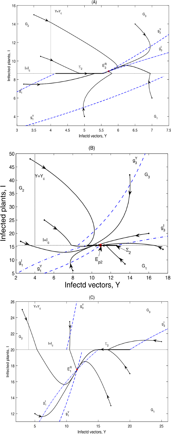

  

  Global dynamics in Case A.13. (A) $E_{3}^{R}$ is globally asymptotically stable. $Y_{c}=4$, $I_{c}=8.65$. (B) $E_{p2}$ is globally asymptotically stable. $Y_{c}=4$, $I_{c}=15.5$. (C) $E_{1}^{R}$ is globally asymptotically stable. $Y_{c}=4$, $I_{c}=20$

• (ii) if $g_{5}< I_{3}^{*}< I_{c}< I_{1}^{*}$, $E_{p2}\in \varSigma _{2}\subset \varOmega _{1}$, $E_{1}$and $E_{3}$are virtual equilibria, denoted by $E_{1}^{V}$and $E_{3}^{V}$, respectively; then $E_{p2}$is globally asymptotically stable; as can be seen in Fig. 5(B);

• (iii) if $g_{5}< I_{3}^{*}< I_{1}^{*}< I_{c}$, $E_{p2}\notin \varSigma _{2}\subset \varOmega _{1}$, $E_{1}$is a real equilibrium, while $E_{3}$is a virtual equilibrium, denoted by $E_{1}^{R}$and $E_{3}^{V}$, respectively; then $E_{1}^{R}$is globally asymptotically stable; as can be seen in Fig. 5(C).

The phase portrait in Fig. 5(A) shows that the infected plants will finally converge to a level above the infected plant threshold value $I_{c}$, while for Fig. 5(B) and (C), the infected plants will finally stabilize at a level equal to or below $I_{c}$.

3.2 Case A.2: $g_{1}< g_{3}< g_{4}< I_{3}^{*}< g_{5}< I_{2}^{*}< I_{1}^{*}$

3.2.1 Case A.21: $I_{c}< g_{4}< g_{5}$

In this case, the discussion is similar to Case A.11, and we omit it.

3.2.2 Case A.22: $g_{4}< I_{c}< g_{5}$

In Case A.22, $E_{1}$ is a virtual equilibrium, denoted by $E_{1}^{V}$. The sliding mode $\varSigma _{1}=\{(Y,I)\in \varOmega _{1}: h_{1}< Y< Y_{c}\}$, $\varSigma _{2}=\{(Y,I)\in \varOmega _{1}: Y_{c}< Y< h_{2}\}$, however, $E_{p1}\notin \varSigma _{1}$. The sliding mode $\varSigma _{3}$ does not exist. From Proposition 2.2, we can obtain the following results.

Theorem 3.4

According to the threshold value $I_{c}$, we have

• (i) if $g_{4}< I_{c}< I_{3}^{*}< g_{5}$, $E_{p2}\notin \varSigma _{2}\subset \varOmega _{1}$, $E_{3}$is a real equilibrium, denoted by $E_{3}^{R}$; then $E_{3}^{R}$is globally asymptotically stable; as can be seen in Fig. 6(A);

  Figure 6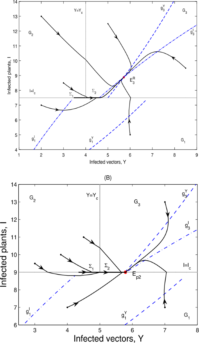

  

  Global dynamics in Case A.22. (A) $E_{3}^{R}$ is globally asymptotically stable. $Y_{c}=4$, $I_{c}=7.5$. (B) $E_{p2}$ is globally asymptotically stable. $Y_{c}=5$, $I_{c}=9$

• (ii) if $g_{4}< I_{3}^{*}< I_{c}< g_{5}$, $E_{p2}\in \varSigma _{2}\subset \varOmega _{1}$, $E_{3}$is a virtual equilibrium, denoted by $E_{3}^{V}$; then $E_{p2}$is globally asymptotically stable; as can be seen in Fig. 6(B).

It can be seen from Fig. 6(A) and (B) that the infected plants will finally converge to a level either above or equal to $I_{c}$.

3.2.3 Case A.23: $g_{4}< g_{5}< I_{c}$

In this case, the sliding mode $\varSigma _{2}=\{(Y,I)\in \varOmega _{1}: h_{1}< Y< h_{2}\}$, while $\varSigma _{1}$ and $\varSigma _{3}$ do not exist. From Proposition 2.2, we can obtain the following results.

Theorem 3.5

According to the threshold value $I_{c}$, we have

• (i) if $g_{4}< I_{3}^{*}< g_{5}< I_{c}< I_{1}^{*}$, $E_{p2}\in \varSigma _{2}\subset \varOmega _{1}$, $E_{1}$and $E_{3}$are virtual equilibria, denoted by $E_{1}^{V}$and $E_{3}^{V}$, respectively; then $E_{p2}$is globally asymptotically stable;

• (ii) if $g_{4}< I_{3}^{*}< g_{5}< I_{1}^{*}< I_{c}$, $E_{p2}\notin \varSigma _{2}\subset \varOmega _{1}$, $E_{1}$is a real equilibrium, while $E_{3}$is a virtual equilibrium, denoted by $E_{1}^{R}$and $E_{3}^{V}$, respectively; then $E_{1}^{R}$is globally asymptotically stable.

The phase portrait in this case is similar to that in Fig. 5(B) and (C), we just omit it.

3.3 Case A.3: $g_{1}< g_{3}< g_{4}< I_{3}^{*}< I_{2}^{*}< g_{5}< I_{1}^{*}$

3.3.1 Case A.31: $I_{c}< g_{4}< g_{5}$

In this case, the discussion is similar to Case A.11, and we omit it.

3.3.2 Case A.32: $g_{4}< I_{c}< g_{5}$

In Case A.32, $E_{1}$ is a virtual equilibrium, denoted by $E_{1}^{V}$. The sliding mode $\varSigma _{1}=\{(Y,I)\in \varOmega _{1}: h_{1}< Y< Y_{c}\}$, $\varSigma _{2}=\{(Y,I)\in \varOmega _{1}: Y_{c}< Y< h_{2}\}$, however, $E_{p1}\notin \varSigma _{1}$. The sliding mode $\varSigma _{3}$ does not exist. From Proposition 2.2, we can obtain the following results.

Theorem 3.6

According to the threshold value $I_{c}$, we have

• (i) if $g_{4}< I_{c}< I_{3}^{*}< g_{5}$, $E_{p2}\notin \varSigma _{2}\subset \varOmega _{1}$, $E_{1}$is a virtual equilibrium, while $E_{3}$is a real equilibrium, denoted by $E_{1}^{V}$and $E_{3}^{R}$, respectively; then $E_{3}^{R}$is globally asymptotically stable;

• (ii) if $g_{4}< I_{3}^{*}< I_{c}< g_{5}$, $E_{p2}\in \varSigma _{2}\subset \varOmega _{1}$, $E_{1}$and $E_{3}$are virtual equilibria, denoted by $E_{1}^{V}$and $E_{3}^{V}$, respectively; then $E_{p2}$is globally asymptotically stable.

The phase portrait in this case is similar to that in Fig. 6, we just omit it.

3.3.3 Case A.33: $g_{4}< g_{5}< I_{c}$

In this case, the discussion is similar to Case A.23 and is omitted here.

4 Global behavior in Case B: $Y_{3}^{*}< Y_{c}< Y_{2}^{*}< Y_{1}^{*}$

In Case B, where $Y_{3}^{*}< Y_{c}< Y_{2}^{*}$, both $E_{2}$ and $E_{3}$ are virtual equilibria, denoted by $E_{2}^{V}$ and $E_{3}^{V}$, respectively. We first present the following lemma according to Proposition 2.4 if Case B is established.

Lemma 4.1

The following formula holds:

$$ Y_{3}^{*}< Y_{c}< Y_{2}^{*}< Y_{1}^{*}\quad \Leftrightarrow \quad I_{3}^{*}< g_{1}< g_{4}< I_{2}^{*}< I_{1}^{*} \quad \textit{and} \quad g_{1}< I_{3}^{*}< g_{4}< I_{2}^{*}< I_{1}^{*}. $$

For $g_{4}< g_{3}< g_{5}< I_{1}^{*}$, we have the following three situations.

• (i) Case B.1: $I_{3}^{*}< g_{1}< g_{4}< g_{3}< g_{5}< I_{2}^{*}< I_{1}^{*}$ ($g_{1}< I_{3}^{*}< g_{4}< g_{3}< g_{5}< I_{2}^{*}< I_{1}^{*}$);

• (ii) Case B.2: $I_{3}^{*}< g_{1}< g_{4}< g_{3}< I_{2}^{*}< g_{5}< I_{1}^{*}$ ($g_{1}< I_{3}^{*}< g_{4}< g_{3}< I_{2}^{*}< g_{5}< I_{1}^{*}$);

• (iii) Case B.3: $I_{3}^{*}< g_{1}< g_{4}< I_{2}^{*}< g_{3}< g_{5}< I_{1}^{*}$ ($g_{1}< I_{3}^{*}< g_{4}< I_{2}^{*}< g_{3}< g_{5}< I_{1}^{*}$).

Note that the results when $g_{1}< I_{3}^{*}$ is the same with $I_{3}^{*}< g_{1}$, hence we only present the situations when $I_{3}^{*}< g_{1}$.

4.1 Case B.1: $I_{3}^{*}< g_{1}< g_{4}< g_{3}< g_{5}< I_{2}^{*}< I_{1}^{*}$

4.1.1 Case B.11: $I_{c}< g_{4}< g_{5}$

In Case B.11, $E_{1}$ is a virtual equilibrium, denoted by $E_{1}^{V}$. The sliding mode $\varSigma _{1}=\{(Y,I)\in \varOmega _{1}: h_{1}< Y< h_{2}\}$, however, $E_{p1}\notin \varSigma _{1}\subset \varOmega _{1}$, while the sliding mode $\varSigma _{2}$ does not exist. The sliding mode $\varSigma _{3}=\{(Y,I)\in \varOmega _{2}: g_{1}< I< g_{2}\}$ if $I_{c}< g_{1}< g_{4}$, while $\varSigma _{3}=\{(Y,I)\in \varOmega _{2}: I_{c}< I< g_{2}\}$ if $g_{1} < I_{c}< g_{4}$, and $E_{p3}\in \varSigma _{3}\subset \varOmega _{2}$. We can get the global asymptotic stability of $E_{p3}$ by excluding the existence of limit cycles.

Theorem 4.1

$E_{p3}$is globally asymptotically stable if $I_{3}^{*}< g_{1}< g_{4}< g_{3}< g_{5}< I_{2}^{*}< I_{1}^{*}$and $I_{c}< g_{4}< g_{5}$.

The phase portrait in Fig. 7 finally stabilizes at a level above the infected plant threshold level $I_{c}$.

Figure 7

$E_{p3}$ is globally asymptotically stable in Case B.11 corresponding to different sliding modes $\varSigma _{3}$. (A1) $Y_{c}=9$, $I_{c}=10$. $\varSigma _{3}=\{(Y,I)\in \varOmega _{2}: g_{1}< I< g_{2}\}$. (A2) $Y_{c}=9$, $I_{c}=12$. $\varSigma _{3}=\{(Y,I)\in \varOmega _{2}: I_{c}< I< g_{2}\}$. (A2) is omitted here

4.1.2 Case B.12: $g_{4}< I_{c}< g_{5}$

In Case B.12, $E_{1}$ is a virtual equilibrium, denoted by $E_{1}^{V}$. The sliding mode $\varSigma _{1}=\{(Y,I)\in \varOmega _{1}: h_{1}< Y< Y_{c}\}$, $\varSigma _{2}=\{(Y,I)\in \varOmega _{1}: Y_{c}< Y< h_{2}\}$, however, $E_{p1}\notin \varSigma _{1}$. The sliding mode $\varSigma _{3}=\{(Y,I)\in \varOmega _{2}: I_{c}< I< g_{2}\}$ if $g_{4}< I_{c}< g_{3}< g_{5}$, while $\varSigma _{3}$ depends on $g_{2}$ and $I_{c}$ if $g_{4}< g_{3}< I_{c}< g_{5}$. $E_{p3}$ is never a pseudoequilibrium even if the sliding mode $\varSigma _{3}$ exists.

Theorem 4.2

According to the threshold value $I_{c}$, we have

• (i) if $g_{4}< I_{c}< g_{3}< g_{5}$, $E_{p2}\notin \varSigma _{2}\subset \varOmega _{1}$, no equilibrium exists in the system. However, all orbits will converge in a finite time to the pseudoattractor $E_{c}=(Y_{c},I_{c})$; as can be seen in Fig. 8(A);

  Figure 8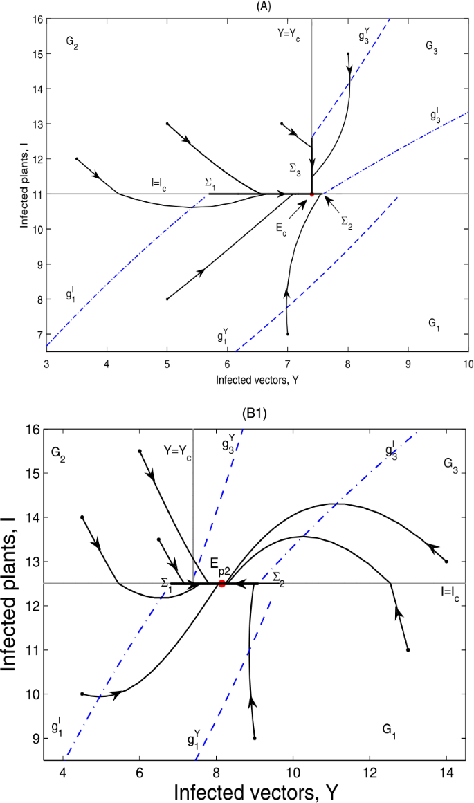

  

  Global dynamics in Case B.12. (A) $E_{c}$ is globally asymptotically stable. $Y_{c}=7.4$, $I_{c}=11$. (B1) $E_{p2}$ is globally asymptotically stable. $Y_{c}=7.4$, $I_{c}=12.5$. $\varSigma _{3}$ does not exist. (B2) $E_{p2}$ is globally asymptotically stable. $Y_{c}=7.4$, $I_{c}=12$. $\varSigma _{3}=\{(Y,I)\in \varOmega _{2}: I_{c}< I< g_{2}\}$. (B2) is omitted here

• (ii) if $g_{4}< g_{3}< I_{c}< g_{5}$, $E_{p2}\in \varSigma _{2}\subset \varOmega _{1}$; then $E_{p2}$is globally asymptotically stable; as can be seen in Fig. 8(B1) and (B2).

It can be seen from Fig. 8 that the infected plants will finally converge to a level equal to $I_{c}$.

4.1.3 Case B.13: $g_{4}< g_{5}< I_{c}$

In this case, the sliding mode $\varSigma _{2}=\{(Y,I)\in \varOmega _{1}: h_{1}< Y< h_{2}\}$, while $\varSigma _{1}$ does not exist. The sliding mode $\varSigma _{3}$ depends on $g_{2}$ and $I_{c}$, however, $E_{p3}$ is never a pseudoequilibrium even if the sliding mode $\varSigma _{3}$ exists. From Proposition 2.2, we can obtain the following results.

Theorem 4.3

According to the threshold value $I_{c}$, we have

• (i) if $g_{4}< g_{3}< g_{5}< I_{c}< I_{1}^{*}$, $E_{p2}\in \varSigma _{2}\subset \varOmega _{1}$, $E_{1}$is a virtual equilibrium, denoted by $E_{1}^{V}$; then $E_{p2}$is globally asymptotically stable; as can be seen in Fig. 9(A1) and (A2);

  Figure 9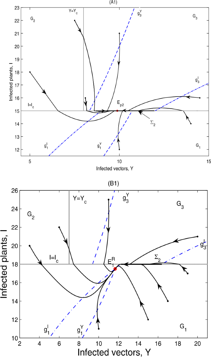

  

  Global dynamics in Case B.13. (A1) $E_{p2}$ is globally asymptotically stable. $Y_{c}=8$, $I_{c}=15$. $\varSigma _{3}$ does not exist. (A2) $E_{p2}$ is globally asymptotically stable. $Y_{c}=9$, $I_{c}=16$. $\varSigma _{3}=\{(Y,I)\in \varOmega _{2}: I_{c}< I< g_{2}\}$. (B1) $E_{1}^{R}$ is globally asymptotically stable. $Y_{c}=7$, $I_{c}=18$. $\varSigma _{3}$ does not exist. (B2) $E_{1}^{R}$ is globally asymptotically stable. $Y_{c}=10$, $I_{c}=18$. $\varSigma _{3}=\{(Y,I)\in \varOmega _{2}: I_{c}< I< g_{2}\}$. (A2) and (B2) are omitted here

• (ii) if $g_{4}< g_{3}< g_{5}< I_{2}^{*}< I_{1}^{*}< I_{c}$, $E_{p2}\notin \varSigma _{2}\subset \varOmega _{1}$, $E_{1}$is a real equilibrium, denoted by $E_{1}^{R}$; then $E_{1}^{R}$is globally asymptotically stable; as can be seen in Fig. 9(B1) and (B2).

It can be seen from Fig. 9 that the infected plants will finally converge to a level equal to or below $I_{c}$.

4.2 Case B.2: $I_{3}^{*}< g_{1}< g_{4}< g_{3}< I_{2}^{*}< g_{5}< I_{1}^{*}$

4.2.1 Case B.21: $I_{c}< g_{4}< g_{5}$

In this case, the discussion is similar to Case B.11 and is omitted here.

4.2.2 Case B.22: $g_{4}< I_{c}< g_{5}$

In Case B.22, $E_{1}$ is a virtual equilibrium, denoted by $E_{1}^{V}$. The sliding mode $\varSigma _{1}=\{(Y,I)\in \varOmega _{1}: h_{1}< Y< Y_{c}\}$, $\varSigma _{2}=\{(Y,I)\in \varOmega _{1}: Y_{c}< Y< h_{2}\}$, however, $E_{p1}\notin \varSigma _{1}$. The sliding mode $\varSigma _{3}=\{(Y,I)\in \varOmega _{2}: I_{c}< I< g_{2}\}$ if $g_{4}< I_{c}< g_{3}$, while $\varSigma _{3}$ depends on $g_{2}$ and $I_{c}$ if $g_{4}< g_{3}< I_{c}$. $E_{p3}$ is never a pseudoequilibrium even if the sliding mode $\varSigma _{3}$ exists.

Theorem 4.4

According to the threshold value $I_{c}$, we have

• (i) if $g_{4}< I_{c}< g_{3}< I_{2}^{*}< g_{5}$, $E_{p2}\notin \varSigma _{2}\subset \varOmega _{1}$, no equilibrium exists in the system. However, all orbits will converge in a finite time to the pseudoattractor $E_{c}=(Y_{c},I_{c})$;

• (ii) if $g_{4}< g_{3}< I_{c}< g_{5}$, $E_{p2}\in \varSigma _{2}\subset \varOmega _{1}$; then $E_{p2}$is globally asymptotically stable.

The phase portrait in this case is similar to that in Fig. 8, we just omit it.

4.2.3 Case B.23: $g_{4}< g_{5}< I_{c}$

In this case, the sliding mode $\varSigma _{2}=\{(Y,I)\in \varOmega _{1}: h_{1}< Y< h_{2}\}$, while $\varSigma _{1}$ does not exist. The sliding mode $\varSigma _{3}$ depends on $g_{2}$ and $I_{c}$, however, $E_{p3}$ is never a pseudoequilibrium even if the sliding mode $\varSigma _{3}$ exists. From Proposition 2.2, we can obtain the following results.

Theorem 4.5

According to the threshold value $I_{c}$, we have

• (i) if $g_{4}< I_{2}^{*}< g_{3}< g_{5}< I_{c}< I_{1}^{*}$, $E_{p2}\in \varSigma _{2}\subset \varOmega _{1}$, $E_{1}$is a virtual equilibrium, denoted by $E_{1}^{V}$; then $E_{p2}$is globally asymptotically stable;

• (ii) if $g_{4}< I_{2}^{*}< g_{3}< g_{5}< I_{1}^{*}< I_{c}$, $E_{p2}\notin \varSigma _{2}\subset \varOmega _{1}$, $E_{1}$is a real equilibrium, denoted by $E_{1}^{R}$; then $E_{1}^{R}$is globally asymptotically stable.

The phase portrait in this case is similar to that in Fig. 9, we just omit it.

4.3 Case B.3: $I_{3}^{*}< g_{1}< g_{4}< I_{2}^{*}< g_{3}< g_{5}< I_{1}^{*}$

4.3.1 Case B.31: $I_{c}< g_{4}< g_{5}$

In this case, the discussion is the same with Case B.11 and is omitted here.

4.3.2 Case B.32: $g_{4}< I_{c}< g_{5}$

In Case B.32, $E_{1}$ is a virtual equilibrium, denoted by $E_{1}^{V}$. The sliding mode $\varSigma _{1}=\{(Y,I)\in \varOmega _{1}: h_{1}< Y< Y_{c}\}$, $\varSigma _{2}=\{(Y,I)\in \varOmega _{1}: Y_{c}< Y< h_{2}\}$, however, $E_{p1}\notin \varSigma _{1}$. The sliding mode $\varSigma _{3}=\{(Y,I)\in \varOmega _{2}: I_{c}< I< g_{2}\}$ if $g_{4}< I_{c}< g_{3}$, while $\varSigma _{3}$ depends on $g_{2}$ and $I_{c}$ if $g_{4}< I_{2}^{*}< g_{3}< I_{c}$. $E_{p3}$ is never a pseudoequilibrium even if the sliding mode $\varSigma _{3}$ exists.

Theorem 4.6

According to the threshold value $I_{c}$, we have

• (i) if $g_{4}< I_{c}< g_{3}< g_{5}$, $E_{p2}\notin \varSigma _{2}\subset \varOmega _{1}$, no equilibrium exists in the system. However, all orbits will converge in a finite time to the pseudoattractor $E_{c}=(Y_{c},I_{c})$;

• (ii) if $g_{4}< I_{2}^{*}< g_{3}< I_{c}< g_{5}$, $E_{p2}\in \varSigma _{2}\subset \varOmega _{1}$; then $E_{p2}$is globally asymptotically stable.

The phase portrait in this case is similar to that in Fig. 8, we just omit it.

4.3.3 Case B.33: $g_{4}< g_{5}< I_{c}$

In this case, the discussion is the same with Case B.23 and is omitted here.

5 Global behavior in Case C: $Y_{3}^{*}< Y_{2}^{*}< Y_{c}< Y_{1}^{*}$

In Case C, where $Y_{3}^{*}< Y_{2}^{*}< Y_{c}< Y_{1}^{*}$, $E_{3}$ is a virtual equilibrium, denoted by $E_{3}^{V}$. We first present the following lemma according to Proposition 2.4 if Case C is established.

Lemma 5.1

The following formula holds

$$ Y_{3}^{*}< Y_{2}^{*}< Y_{c}< Y_{1}^{*}\quad \Leftrightarrow \quad I_{3}^{*}< I_{2}^{*}< g_{4}< g_{1}< g_{3}< g_{5}< I_{1}^{*}. $$

5.1 Case C.1: $I_{c}< g_{4}< g_{5}$

In Case C.1, $E_{1}$ is a virtual equilibrium, denoted by $E_{1}^{V}$. The sliding mode $\varSigma _{1}=\{(Y,I)\in \varOmega _{1}: h_{1}< Y< h_{2}\}$, while the sliding mode $\varSigma _{2}$ does not exist. The sliding mode $\varSigma _{3}=\{(Y,I)\in \varOmega _{2}: g_{1}< I< g_{2}\}$ and $E_{p3}$ is never a pseudoequilibrium.

Theorem 5.1

According to the threshold value $I_{c}$, we have

• (i) if $I_{c}< I_{2}^{*}< g_{4}$, $E_{p1}\notin \varSigma _{1}\subset \varOmega _{1}$, $E_{2}$is a real equilibrium, denoted by $E_{2}^{R}$; then $E_{2}^{R}$is globally asymptotically stable; as can be seen in Fig. 10(A);

  Figure 10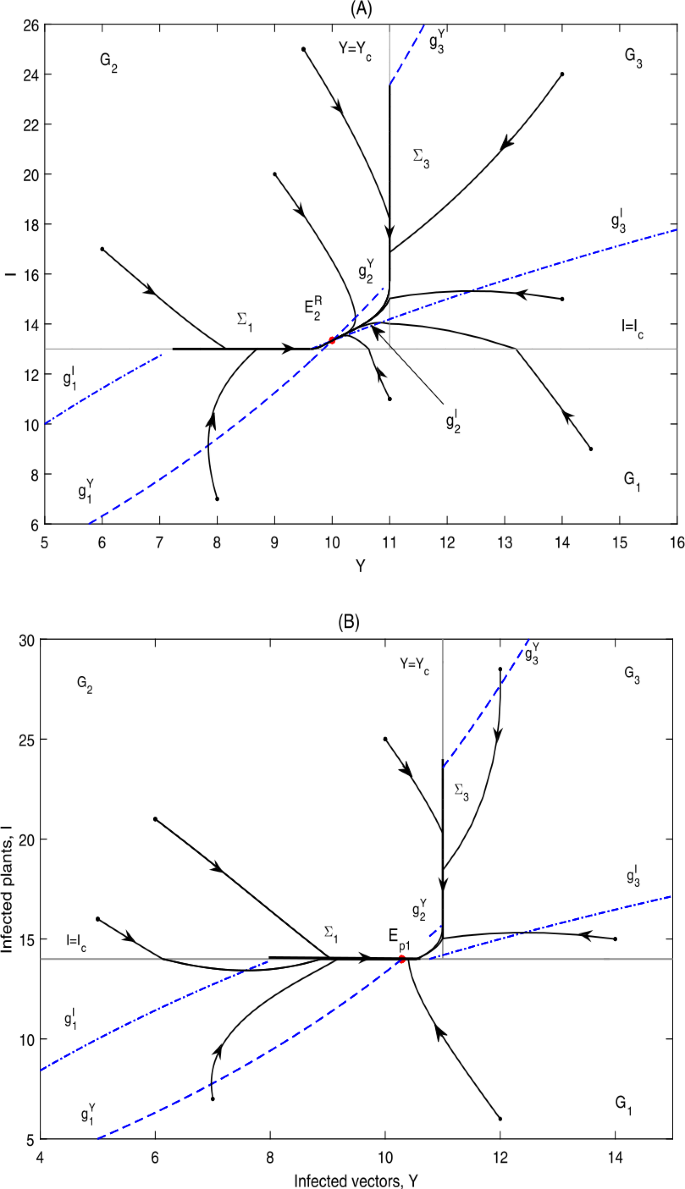

  

  Global dynamics in Case C.1. (A) $E_{2}^{R}$ is globally asymptotically stable. $Y_{c}=11$, $I_{c}=13$. (B) $E_{p1}$ is globally asymptotically stable. $Y_{c}=11$, $I_{c}=14$

• (ii) if $I_{2}^{*}< I_{c}< g_{4}$, $E_{p1}\in \varSigma _{1}\subset \varOmega _{1}$, $E_{2}$is a virtual equilibrium, denoted by $E_{2}^{V}$; then $E_{p1}$is globally asymptotically stable; as can be seen in Fig. 10(B).

It can be seen from Fig. 10 that the infected plants will finally converge to a level above or equal to $I_{c}$.

5.2 Case C.2: $g_{4}< I_{c}< g_{5}$

In Case C.2, both $E_{1}$ and $E_{2}$ are virtual equilibria, denoted by $E_{1}^{V}$ and $E_{2}^{V}$, respectively. The sliding mode $\varSigma _{1}=\{(Y,I)\in \varOmega _{1}: h_{1}< Y< Y_{c}\}$, $\varSigma _{2}=\{(Y,I)\in \varOmega _{1}: Y_{c}< Y< h_{2}\}$. $E_{p3}$ is never a pseudoequilibrium even if the sliding mode $\varSigma _{3}$ exists.

Theorem 5.2

According to the threshold value $I_{c}$, we have

• (i) if $g_{4}< I_{c}< g_{1}< g_{3}< g_{5}$, $\varSigma _{3}=\{(Y,I)\in \varOmega _{2}: g_{1}< I< g_{2}\}$, $E_{p1}\in \varSigma _{1}\subset \varOmega _{1}$, $E_{p2}\notin \varSigma _{2}\subset \varOmega _{1}$; then $E_{p1}$is globally asymptotically stable; as can be seen in Fig. 11(A);

  Figure 11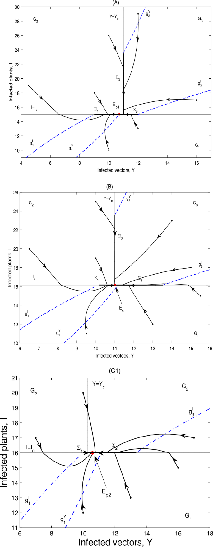

  

  Global dynamics in Case C.2. (A) $E_{p1}$ is globally asymptotically stable. $Y_{c}=11$, $I_{c}=15$. (B) $E_{c}$ is globally asymptotically stable. $Y_{c}=11$, $I_{c}=16.15$. (C1) $E_{p2}$ is globally asymptotically stable. $Y_{c}=10.3$, $I_{c}=16$. $\varSigma _{3}$ does not exist. (C2) $E_{p2}$ is globally asymptotically stable. $Y_{c}=10.7$, $I_{c}=16.5$. $\varSigma _{3}=\{(Y,I)\in \varOmega _{2}: I_{c}< I< g_{2}\}$. (C2) is omitted here

• (ii) if $g_{4}< g_{1}< I_{c}< g_{3}< g_{5}$, $\varSigma _{3}=\{(Y,I)\in \varOmega _{2}: I_{c}< I< g_{2}\}$, $E_{p1}\notin \varSigma _{1}\subset \varOmega _{1}$, $E_{p2}\notin \varSigma _{2}\subset \varOmega _{1}$, no equilibrium exists in the system. However, all orbits will converge in a finite time to the pseudoattractor $E_{c}=(Y_{c},I_{c})$; as can be seen in Fig. 11(B);

• (iii) if $g_{4}< g_{1}< g_{3}< I_{c}< g_{5}$, $\varSigma _{3}$depends on $g_{2}$and $I_{c}$, $E_{p1}\notin \varSigma _{1}\subset \varOmega _{1}$, $E_{p2}\in \varSigma _{2}\subset \varOmega _{1}$; then $E_{p2}$is globally asymptotically stable; as can be seen in Fig. 11(C1) and (C2).

It can be seen from Fig. 11 that the infected plants will finally converge to a level equal to $I_{c}$.

Remark

Note that when $Y_{3}^{*}< Y_{c}< Y_{2}^{*}$, $g_{4}< I_{c}< g_{3}$ or $Y_{2}^{*}< Y_{c}< Y_{1}^{*}$, $g_{1}< I_{c}< g_{3}$, all of $E_{1}^{V}$, $E_{2}^{V}$ and $E_{3}^{V}$ are virtual equilibria, while no pseudoequilibrium exists, then the solutions of the system will finally stabilize at the pseudoattractor $E_{c}=(S_{c},I_{c})$, as can be seen in Fig. 8(A) and Fig. 11(B). When the threshold values $Y_{c}$ and $I_{c}$ are chosen from other regions, the system will finally stabilize at either a real equilibrium or a stable pseudoequilibrium. For more complicated dynamics of non-smooth systems including the intersection $E_{c}(S_{c},I_{c})$, the interested reader can refer to [29–33].

5.3 Case C.3: $g_{4}< g_{5}< I_{c}$

In this case, $E_{2}$ is a virtual equilibrium, denoted by $E_{2}^{V}$. The sliding mode $\varSigma _{2}=\{(Y,I)\in \varOmega _{1}: h_{1}< Y< h_{2}\}$, while $\varSigma _{1}$ does not exist. The sliding mode $\varSigma _{3}$ depends on $g_{c}$ and $I_{c}$, however, $E_{p3}$ is never a pseudoequilibrium even if the sliding mode $\varSigma _{3}$ exists. From Proposition 2.2, we can obtain the following results.

Theorem 5.3

According to the threshold value $I_{c}$, we have

• (i) if $g_{5}< I_{c}< I_{1}^{*}$, $E_{p2}\in \varSigma _{2}\subset \varOmega _{1}$, $E_{1}$is a virtual equilibrium, denoted by $E_{1}^{V}$; then $E_{p2}$is globally asymptotically stable; as can be seen in Fig. 12(A1) and (A2);

  Figure 12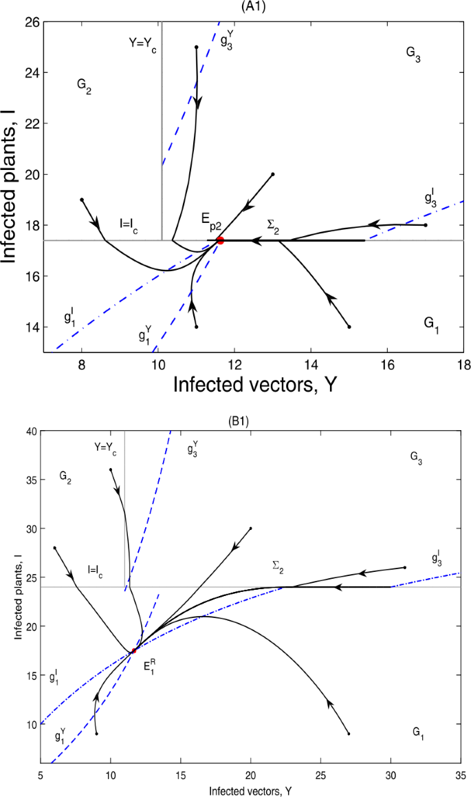

  

  Global dynamics in Case C.3. (A1) $E_{p2}$ is globally asymptotically stable. $Y_{c}=10.1$, $I_{c}=17.4$. $\varSigma _{3}$ does not exist. (A2) $E_{p2}$ is globally asymptotically stable. $Y_{c}=10.5$, $I_{c}=17$. $\varSigma _{3}=\{(Y,I)\in \varOmega _{2}: I_{c}< I< g_{2}\}$. (B1) $E_{1}^{R}$ is globally asymptotically stable. $Y_{c}=11$, $I_{c}=24$. $\varSigma _{3}$ does not exist. (B2) $E_{1}^{R}$ is globally asymptotically stable. $Y_{c}=11$, $I_{c}=19$. $\varSigma _{3}=\{(Y,I)\in \varOmega _{2}: I_{c}< I< g_{2}\}$. (A2) and (B2) are omitted here

• (ii) if $g_{5}< I_{1}^{*}< I_{c}$, $E_{p2}\notin \varSigma _{2}\subset \varOmega _{1}$, $E_{1}$is a real equilibrium, denoted by $E_{1}^{R}$; then $E_{1}^{R}$is globally asymptotically stable; as can be seen in Fig. 12(B1) and (B2).

It can be seen from Fig. 12 that the infected plants will finally converge to a level equal to or below $I_{c}$.

6 Global behavior in Case D: $Y_{3}^{*}< Y_{2}^{*}< Y_{1}^{*}< Y_{c}$

In Case D, where $Y_{3}^{*}< Y_{2}^{*}< Y_{c}$, $E_{3}$ is a virtual equilibrium, denoted by $E_{3}^{V}$. We first present the following lemma according to Proposition 2.4 if Case D is established.

Lemma 6.1

The following formula holds:

$$ Y_{3}^{*}< Y_{2}^{*}< Y_{1}< Y_{c}^{*}\quad \Leftrightarrow \quad I_{3}^{*}< I_{2}^{*}< I_{1}^{*}< g_{5}< g_{3}< g_{1}. $$

For $I_{2}^{*}< g_{4}< g_{5}$, we have the following two situations.

• (i) Case D.1: $I_{3}^{*}< I_{2}^{*}< g_{4}< I_{1}^{*}< g_{5}< g_{3}< g_{1}$;

• (ii) Case D.2: $I_{3}^{*}< I_{2}^{*}< I_{1}^{*}< g_{4}< g_{5}< g_{3}< g_{1}$.

6.1 Case D.1: $I_{3}^{*}< I_{2}^{*}< g_{4}< I_{1}^{*}< g_{5}< g_{3}< g_{1}$

6.1.1 Case D.11: $I_{c}< g_{4}< g_{5}$

In Case D.11, $E_{1}$ is a virtual equilibrium, denoted by $E_{1}^{V}$. The sliding mode $\varSigma _{1}=\{(Y,I)\in \varOmega _{1}: h_{1}< Y< h_{2}\}$, while the sliding mode $\varSigma _{2}$ does not exist. The sliding mode $\varSigma _{3}=\{(Y,I)\in \varOmega _{2}: g_{1}< I< g_{2}\}$ and $E_{p3}$ is never a pseudoequilibrium.

Theorem 6.1

According to the threshold value $I_{c}$, we have

• (i) if $I_{c}< I_{2}^{*}< g_{4}$, $E_{p1}\notin \varSigma _{1}\subset \varOmega _{1}$, $E_{2}$is a real equilibrium, denoted by $E_{2}^{R}$; then $E_{2}^{R}$is globally asymptotically stable; as can be seen in Fig. 13(A);

  Figure 13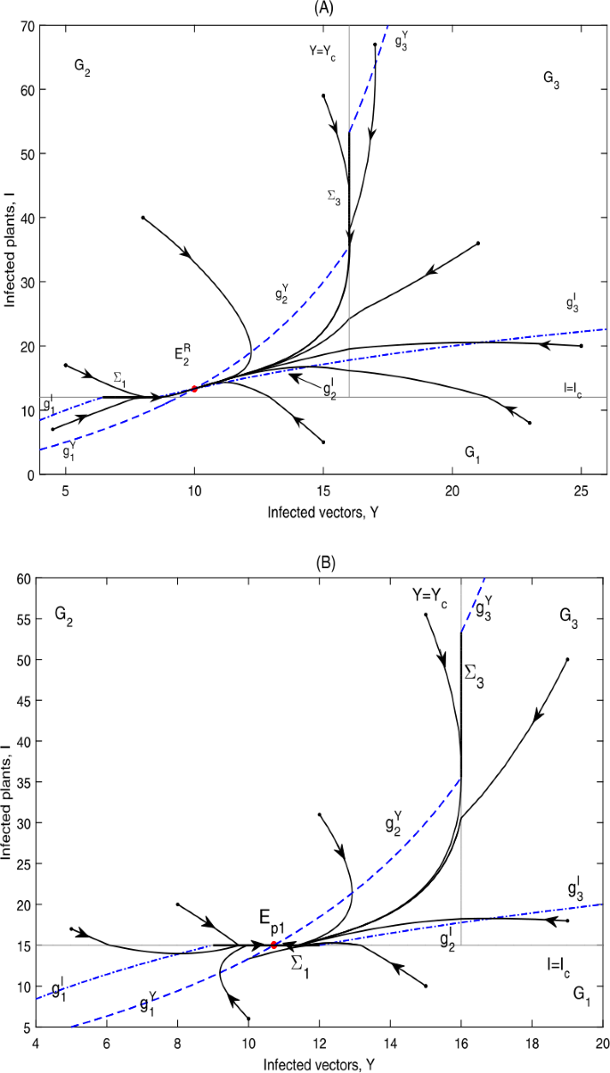

  

  Global dynamics in Case D.11. (A) $E_{2}^{R}$ is globally asymptotically stable. $Y_{c}=16$, $I_{c}=12$. (B) $E_{p1}$ is globally asymptotically stable. $Y_{c}=16$, $I_{c}=15$

• (ii) if $I_{2}^{*}< I_{c}< g_{4}$, $E_{p1}\in \varSigma _{1}\subset \varOmega _{1}$, $E_{2}$is a virtual equilibrium, denoted by $E_{2}^{V}$; then $E_{p1}$is globally asymptotically stable; as can be seen in Fig. 13(B).

It can be seen from Fig. 13 that the infected plants will finally converge to a level above or equal to $I_{c}$.

6.1.2 Case D.12: $g_{4}< I_{c}< g_{5}$

In Case D.12, $E_{2}$ is a virtual equilibrium, denoted by $E_{2}^{V}$. The sliding mode $\varSigma _{1}=\{(Y,I)\in \varOmega _{1}: h_{1}< Y< Y_{c}\}$, $\varSigma _{2}=\{(Y,I)\in \varOmega _{1}: Y_{c}< Y< h_{2}\}$, and $\varSigma _{3}=\{(Y,I)\in \varOmega _{2}: g_{1}< I< g_{2}\}$. However, $E_{p3}$ is never a pseudoequilibrium.

Theorem 6.2

According to the threshold value $I_{c}$, we have

• (i) if $g_{4}< I_{c}< I_{1}^{*}< g_{5}$, $E_{p1}\in \varSigma _{1}\subset \varOmega _{1}$, $E_{p2}\notin \varSigma _{2}\subset \varOmega _{1}$, $E_{1}$is a virtual equilibrium, denoted by $E_{1}^{V}$; then $E_{p1}$is globally asymptotically stable; as can be seen in Fig. 14(A);

  Figure 14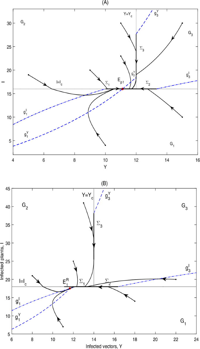

  

  Global dynamics in Case D.12. (A) $E_{p1}$ is globally asymptotically stable. $Y_{c}=12$, $I_{c}=16$. (B) $E_{1}^{R}$ is globally asymptotically stable. $Y_{c}=14$, $I_{c}=18$

• (ii) if $g_{4}< I_{1}^{*}< I_{c}< g_{5}$, $E_{p1}\notin \varSigma _{1}\subset \varOmega _{1}$, $E_{p2}\notin \varSigma _{2}\subset \varOmega _{1}$, $E_{1}$is a real equilibrium, denoted by $E_{1}^{R}$; then $E_{1}^{R}$is globally asymptotically stable; as can be seen in Fig. 14(B).

It can be seen from Fig. 14 that the infected plants will finally converge to a level below or equal to $I_{c}$.

6.1.3 Case D.13: $g_{4}< g_{5}< I_{c}$

In this case, $E_{1}$ is a real equilibrium, $E_{2}$ is a virtual equilibrium, denoted by $E_{1}^{R}$ and $E_{2}^{V}$, respectively. The sliding mode $\varSigma _{2}=\{(Y,I)\in \varOmega _{1}: h_{1}< Y< h_{2}\}$, while $\varSigma _{1}$ does not exist, $E_{p2}\notin \varSigma _{2}\subset \varOmega _{1}$. $\varSigma _{3}=\{(Y,I)\in \varOmega _{2}: g_{1}< I< g_{2}\}$ if $g_{5}< I_{c}< g_{1}$, while $\varSigma _{3}$ depends on $g_{2}$ and $I_{c}$ if $g_{1}< I_{c}$. However, $E_{p3}$ is never a pseudoequilibrium. According to Proposition 2.2, we can obtain the following result.

Theorem 6.3

$E_{1}^{R}$is globally asymptotically stable if $I_{3}^{*}< I_{2}^{*}< g_{4}< I_{1}^{*}< g_{5}< g_{3}< g_{1}$and $g_{4}< g_{5}< I_{c}$.

As can be seen in Fig. 15, the phase portrait will finally stabilize at a level below the infected threshold value $I_{c}$.

Figure 15

$E_{1}^{R}$ is globally asymptotically stable in Case D.13 corresponding to different sliding modes $\varSigma _{3}$. (A1) $Y_{c}=15$, $I_{c}=25$. $\varSigma _{3}=\{(Y,I)\in \varOmega _{2}: g_{1}< I< g_{2}\}$. (A2) $Y_{c}=13$, $I_{c}=26$. $\varSigma _{3}=\{(Y,I)\in \varOmega _{2}: I_{c}< I< g_{2}\}$. (A3) $Y_{c}=12$, $I_{c}=28$. $\varSigma _{3}$ does not exist. (A2) and (A3) are omitted here

6.2 Case D.2: $I_{3}^{*}< I_{2}^{*}< I_{1}^{*}< g_{4}< g_{5}< g_{3}< g_{1}$

6.2.1 Case D.21: $I_{c}< g_{4}< g_{5}$

In Case D.21, the sliding mode $\varSigma _{1}=\{(Y,I)\in \varOmega _{1}: h_{1}< Y< h_{2}\}$, while the sliding mode $\varSigma _{2}$ does not exist. The sliding mode $\varSigma _{3}=\{(Y,I)\in \varOmega _{2}: g_{1}< I< g_{2}\}$ and $E_{p3}$ is never a pseudoequilibrium.

Theorem 6.4

According to the threshold value $I_{c}$, we have

• (i) if $I_{c}< I_{2}^{*}< I_{1}^{*}< g_{4}$, $E_{p1}\notin \varSigma _{1}\subset \varOmega _{1}$, $E_{1}$is a virtual equilibrium, $E_{2}$is a real equilibrium, denoted by $E_{1}^{V}$and $E_{2}^{R}$, respectively; then $E_{2}^{R}$is globally asymptotically stable;

• (ii) if $I_{2}^{*}< I_{c}< I_{1}^{*}< g_{4}$, $E_{p1}\in \varSigma _{1}\subset \varOmega _{1}$, both $E_{1}$and $E_{2}$are virtual equilibria, denoted by $E_{1}^{V}$and $E_{2}^{V}$, respectively; then $E_{p1}$is globally asymptotically stable;

• (iii) if $I_{2}^{*}< I_{1}^{*}< I_{c}< g_{4}$, $E_{p1}\notin \varSigma _{1}\subset \varOmega _{1}$, $E_{1}$is a real equilibrium, $E_{2}$is a virtual equilibrium, denoted by $E_{1}^{R}$and $E_{2}^{V}$, respectively; then $E_{1}^{R}$is globally asymptotically stable; as can be seen in Fig. 16.

  Figure 16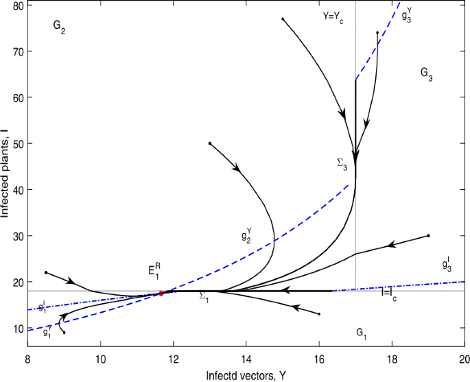

  

  $E_{1}^{R}$ is globally asymptotically stable in Case D.21. $Y_{c}=17$, $I_{c}=18$

The phase portrait of Theorem 6.4 (i) and (ii) is similar to that in Fig. 13, here we just omit it. $E_{1}^{R}$ is globally asymptotically stable as shown in Fig. 16.

6.2.2 Case D.22: $g_{4}< I_{c}< g_{5}$

In Case D.22, $E_{1}$ is a real equilibrium, $E_{2}$ is a virtual equilibrium, denoted by $E_{1}^{R}$ and $E_{2}^{V}$, respectively. The sliding mode $\varSigma _{1}=\{(Y,I)\in \varOmega _{1}: h_{1}< Y< Y_{c}\}$, $\varSigma _{2}=\{(Y,I)\in \varOmega _{1}: Y_{c}< Y< h_{2}\}$, and $\varSigma _{3}=\{(Y,I)\in \varOmega _{2}: g_{1}< I< g_{2}\}$. However, $E_{p1}\notin \varSigma _{1}\subset \varOmega _{1}$, $E_{p2}\notin \varSigma _{2}\subset \varOmega _{1}$, $E_{p3}$ is never a pseudoequilibrium.

Theorem 6.5

$E_{1}^{R}$is globally asymptotically stable if $I_{3}^{*}< I_{2}^{*}< I_{1}^{*}< g_{4}< g_{5}< g_{3}< g_{1}$and $g_{4}< I_{c}< g_{5}$.

The phase portrait in this case is similar to that in Fig. 14(B), we just omit it.

6.2.3 Case D.23: $g_{4}< g_{5}< I_{c}$

In this case, the discussion is similar to Case D.13 and is omitted here.

7 Conclusion and discussion

In this work, we proposed a Filippov–type vector-borne plant disease model by taking roguing infected plants and spraying insecticides into account. Since roguing and vector control are two of the most applicable and effective strategies in controlling plant disease transmission, it is also essential to relieve the economical devastation for growers and the damage to the environment, human health and natural enemies. Hence, we here take the threshold policy by choosing the numbers of infected plants and vectors as reference indices. That is, we take no control strategy if the number of infected plants is less than an infected plant threshold level $I_{c}$; further, we remove infected plants at a rate q once the number of infected plants exceeds $I_{c}$; meanwhile, we spay pesticides if the number of infected vectors exceeds the infected vector threshold level $Y_{c}$, which results in an induced death rate v for the infected vectors. The main analytical results obtained are summarized in Table 1, with the following biological implications.

• (I) For these cases, all trajectories of system (1) with (2) will stabilize at a globally asymptotically stable equilibrium ($E_{3}^{R}$, $E_{2}^{R}$ or $E_{p3}$) that lies above the infected threshold value $I_{c}$ (see Figs. 4, 5(A), 6(A), 7, 10(A), 13(A)). Hence, it is impossible to avoid an epidemic for this situation. Note that, provided that the infected plant threshold value $I_{c}< I_{2}^{*}$, then regardless of the infected vector threshold value $Y_{c}$, this situation will meet.

• (II) For these choices of $Y_{c}$ and $I_{c}$, all orbits of system (1) with (2) will stabilize at either the pseudoequilibrium on $I=I_{c}$ ($E_{p1}$ or $E_{p2}$) or the pseudoattractor $E_{c}=(Y_{c},I_{c})$ as displayed in Figs. 5(B), 6(B), 8, 9(A1) and (A2), 10(B), 11, 12(A1) and (A2), 13(B), 14(A). Hence the number of infected plants will eventually converge to a level equal to $I_{c}$. Thus there is no risk of an epidemic. Note that in these situations, the infected plant threshold value $I_{c}$ mainly lies between $I_{2}^{*}$ and $I_{1}^{*}$.

• (III) If the infected plant threshold value $I_{c}$ is sufficiently high, that is, $I_{c}>I_{1}^{*}$, then system (1) with (2) will converge to the unique globally asymptotically stable equilibrium $E_{1}^{R}$ that lies below $I_{c}$, regardless of the infected threshold value $Y_{c}$, as shown in Figs. 5(C), 9(B1) and (B2), 12(B1) and (B2), 14(B), 15, 16. So the number of infected plants will eventually stabilize at a level below $I_{c}$. Therefore, our control objective to reduce the number of infected plants below the infected threshold value $I_{c}$ can be achieved eventually.

Table 1 Global dynamics of system (1) with (2) summarized from Sects. 3, 4, 5 and 6

From Table 1 and the above three cases, we can see that the phrase portraits of system (1) with (2) has three destinations, the first one is the unique endemic equilibrium $E_{i}$ of the subsystem in $G_{i}$; the second one is the pseudoequilibrium $E_{pi}$ on the three sliding modes $\varSigma _{i}$, $i=1,2,3$; and the third one is the pseudoattractor $E_{c}=(Y_{c},I_{c})$. The different results depend on different choices of the infected plant and vector threshold levels $I_{c}$ and $Y_{c}$, which shows the importance of the choices of the threshold values. The result in Case (I) indicates that, for these choices of the threshold values $I_{c}$ and $Y_{c}$, it is a waste of resources to take control strategy. The results in Cases (II) and (III) indicate that these choices of the threshold values $I_{c}$ and $Y_{c}$ can finally achieve our objective to drive the infected plants to a level below or equal to a desired level $I_{c}$. Hence our findings can provide some theoretical suggestions on when and whether to take control strategies according to the threshold policy.

Note that in this work we assumed the roguing rate of the infected plants is the same once the number of infected plants exceeds the infected plant threshold value $I_{c}$. However, the roguing rate when $Y>Y_{c}$ may be larger than the case when $Y< Y_{c}$, for more infected vectors will infect more plants which results in a more severe transmission. We also assumed bilinear incidence rate with the assumption of homogeneous contact, but other possibilities should be modeled. All of these will be our future work.

References

Jeger, M.J., Holt, J., van den Bosch, F., Madden, L.V.: Epidemiology of insect-transmitted plant viruses: modelling disease dynamics and control interventions. Physiol. Entomol. 29, 291–304 (2004)
Jackson, M., Chen, B.: A model of biological control of plant virus propagation with delays. J. Comput. Appl. Math. 330, 855–865 (2018)
Fereres, A.: Insect vectors as drivers of plant virus emergence. Curr. Opin. Virol. 10, 42–46 (2015)
Thresh, J.M.: Control of plant virus diseases in sub-Saharan Africa: the possibility and feasibility of an integrated approach. Afr. Crop Sci. J. 11, 199–223 (2003)
Thresh, J.M., Cooter, R.J.: Strategies for controlling cassava mosaic disease in Africa. Plant Pathol. 54, 587–614 (2005)
van den Bosch, F., Jeger, M.J., Gilligan, C.A.: Disease control and its selection for damaging plant virus strains in vegetatively propagated staple food crops: a theoretical assessment. Proc. - Royal Soc., Biol. Sci. 274, 11–18 (2007)
Zhao, T.T., Xiao, Y.N.: Plant disease models with nonlinear impulsive cultural control strategies for vegetatively propagated plants. Math. Comput. Simul. 107, 61–91 (2015)
Jeger, M.J., Madden, L.V., van den Bosch, F.: Plant virus epidemiology: applications and prospects for mathematical modeling and analysis to improve understanding and disease control. Plant Dis. 102(5), 837–854 (2018)
Hu, J., Sui, G., Lv, X., Li, X.: Fixed-time control of delayed neural networks with impulsive perturbations. Nonlinear Anal., Model. Control 23(6), 904–920 (2018)
Tang, S.Y., Xiao, Y.N., Chen, L.S., et al.: Integrated pest management models and their dynamical behaviour. Bull. Math. Biol. 67, 115–135 (2005)
Tang, S.Y., Xiao, Y.N., Cheke, R.A.: Dynamical analysis of plant disease models with cultural control strategies and economic thresholds. Math. Comput. Simul. 80, 894–921 (2010)
Yang, X., Li, X., Xi, Q., Duan, P.: Review of stability and stabilization for impulsive delayed systems. Math. Biosci. Eng. 15(6), 1495–1515 (2018)
Jackson, M., Chen, B.: Modeling plant virus propagation with seasonality. J. Comput. Appl. Math. 345, 310–319 (2019)
Shi, R., Zhao, H., Tang, S.: Global dynamic analysis of a vector-borne plant disease model. Adv. Differ. Equ. 2014, 59 (2014)
Gao, S.J., Xia, L.J., Liu, Y., Xie, D.H.: A plant virus disese model with periodic environment and pulse roguing. Stud. Appl. Math. 136, 357–381 (2015)
van den Bosch, F., Jeger, M.J.: The management of African cassava mosaic virus disease. Quantitative methods for life and Earth. In: Proceedings of Biometrics Conference Wageningen UR, 20th June (2001)
Jeger, M.J., van Den Bosch, F., Madden, L.V., Holt, J.: A model for analysing plant-virus transmission characteristics and epidemic development. Math. Med. Biol. 15, 1–18 (1998)
Zhao, T.T., Xiao, Y.N., Smith R.J.: Non-smooth plant disease models with economic thresholds. Math. Biosci. 241(1), 34–48 (2013)
Wang, J.F., Zhang, F.Q., Wang, L.: Equilibrium, pseudoequilibrium and sliding-mode heteroclinic orbit in a Filippov-type plant disease model. Nonlinear Anal., Real World Appl. 31, 308–324 (2016)
Filippov, A.: Differential Equations with Discontinuous Righthand Sides. Kluwer Academic, Dordrecht (1988)
Kuznetsov, Y.A., Rinaldi, S., Gragnani, A.: One parameter bifurcations in planar Filippov systems. Int. J. Bifurc. Chaos 13, 2157–2188 (2003)
Chen, C., Kang, Y.M., Smith R.J.: Sliding motion and global dynamics of a Filippov fire-blight model with economic thresholds. Nonlinear Anal., Real World Appl. 39, 492–519 (2018)
Chen, C., Li, C.T., Kang, Y.M.: Modelling the effects of cutting off infected branches and replanting on fire-blight transmission using Filippov systems. J. Theor. Biol. 439, 127–140 (2018)
van den Driessche, P., Watmough, J.: Reproduction numbers and sub-threshold endemic equilibria for compartmental models of disease transmission. Math. Biosci. 180, 29–48 (2002)
Leine, R.I.: Bifurcations in Discontinuous Mechanical Systems of Filippov-Type. The Universiteitsdrukkerij TU Eindhoven, The Netherlands (2000)
Leine, R.I., van Campen, D.H., van de Vrande, B.L.: Bifurcations in nonlinear discontinuous systems. Nonlinear Dyn. 23, 105–164 (2000)
Xiao, Y., Xu, X., Tang, S.: Sliding mode control of outbreaks of emerging infectious diseases. Bull. Math. Biol. 74, 2403–2422 (2012)
Yang, Y., Wang, L.: Global dynamics and rich sliding motion in an avian-only Filippov system in combating avian influenza. Int. J. Bifurc. Chaos 30(1), 2050008 (2020)
Jeffrey, M.R.: Dynamics at a switching intersection: hierarchy, isonomy, and multiple-sliding. SIAM J. Appl. Dyn. Syst. 13, 1082–1105 (2014)
Liu, X., Cao, J., Yu, W., Song, Q.: Nonsmooth finite-time synchronization of switched coupled neural networks. IEEE Trans. Cybern. 46(10), 2360–2371 (2016)
Liu, X., Su, H., Chen, M.Z.Q.: A switching approach to designing finite-time synchronization controllers of coupled neural networks. IEEE Trans. Neural Netw. Learn. Syst. 27(2), 471–482 (2016)
Yang, D., Li, X., Shen, J., Zhou, Z.: State-dependent switching control of delayed switched systems with stable and unstable modes. Math. Methods Appl. Sci. 41(16), 6968–6983 (2018)
Li, X., Yang, X., Huang, T.: Persistence of delayed cooperative models: impulsive control method. Appl. Math. Comput. 342, 130–146 (2019)
Acknowledgements
Not applicable.
Availability of data and materials
Funding
National Natural Science Foundation of China (NSFC 11401349) and the Foundation for Outstanding Young Scientist in Shandong Province (BS2014SF008).
Author information
Authors and Affiliations
Contributions
In this research work, YY contributed significantly to analysis and manuscript preparation. TZ performed the numerical simulations. All authors read and approved the final manuscript.
Corresponding author
Ethics declarations
Competing interests
The authors declare that they have no competing interests.
Rights and permissions
Open Access This article is licensed under a Creative Commons Attribution 4.0 International License, which permits use, sharing, adaptation, distribution and reproduction in any medium or format, as long as you give appropriate credit to the original author(s) and the source, provide a link to the Creative Commons licence, and indicate if changes were made. The images or other third party material in this article are included in the article’s Creative Commons licence, unless indicated otherwise in a credit line to the material. If material is not included in the article’s Creative Commons licence and your intended use is not permitted by statutory regulation or exceeds the permitted use, you will need to obtain permission directly from the copyright holder. To view a copy of this licence, visit http://creativecommons.org/licenses/by/4.0/.
About this article
Cite this article
Yang, Y., Zhang, T. Modeling plant virus propagation with Filippov control. Adv Differ Equ 2020, 465 (2020). https://doi.org/10.1186/s13662-020-02921-5
Received:
Accepted:
Published:
DOI: https://doi.org/10.1186/s13662-020-02921-5