- Research
- Open access
- Published:
Five semi analytical and numerical simulations for the fractional nonlinear space-time telegraph equation
Advances in Difference Equations volume 2021, Article number: 227 (2021)
Abstract
The accuracy of analytical obtained solutions of the fractional nonlinear space–time telegraph equation that has been constructed in (Hamed and Khater in J. Math., 2020) is checked through five recent semi-analytical and numerical techniques. Adomian decomposition (AD), El Kalla (EK), cubic B-spline (CBS), extended cubic B-spline (ECBS), and exponential cubic B-spline (ExCBS) schemes are used to explain the matching between analytical and approximate solutions, which shows the accuracy of constructed traveling wave solutions. In 1880, Oliver Heaviside derived the considered model to describe the cutting-edge or voltage of an electrified transmission. The matching between solutions has been explained by plotting them in some different sketches.
1 Introduction
Recently, the nonlinearity has been used in distinct fields such as the neural network [2], infectious disease epidemiology [3], plasma physics [4], thermodynamics [5], optic physics [6], population ecology [7], biology and mechanics of fluids [8, 9]. Defining empirically function and parameters in formulating the nonlinear phenomena in nonlinear evolution equations and systems provides reliable data that explain more about dynamic behavior processes and complicated physical ones [10, 11]. Many physicists and mathematicians have focused their attention on formulating some nonlinear phenomena to demonstrate their characterization of undiscovered models [12–14]. Deriving accurate analytical, semi-analytical, approximate techniques has taken more attention of many researchers; consequently, many distinct techniques have been derived, such as [15–20].
Nowadays, based on the integer-order derivative’s failure to show the nonlocal property of the investigated model, many nonlinear phenomena have been formulated in fractional forms [21–23]. Therefore, many fractional derivative operators have been mathematically formulated, such as Atangana–Baleanu fractional operator, the conformal fractional, Caputo fractional, Riemann–Liouville, Caputo–Fabrizio fractional derivative definitions [24–26], to transform the fractional nonlinear partial differential equations to nonlinear ordinary differential ones [27, 28].
In this context, this paper investigates the fractional nonlinear telegraph equation that is used to describe the transmission of the voltage standard [29]. This mathematical model is considered as a primary icon in the electromagnetic waves’ area. The fractional model of this model is given by [30–32]
where b, d are arbitrary constants, while \(\mathcal{D}=\mathcal{D}(x,t)\). Employing the conformable fractional wave transformation with the next form \(\mathcal{Q}(x,t)=\mathcal{S}(\mathfrak{T})\), \(\mathfrak{T}= \frac{a x^{\alpha }}{\alpha }-\frac{c t^{\alpha }}{\alpha }\), where a, c are arbitrary constants, converts Eq. (1) into
The structure of the paper for the rest of its sections is ordered as follows: Sect. 2 investigates the approximate solutions of the considered fractional nonlinear model. Section 3 studies our obtained solutions to show the matching between the computational and numerical solutions, which shows the accuracy of our solutions. Moreover, this section aims to show the originality of our solutions by comparing them with other previously obtained solutions. Section 4 gives the conclusion.
2 Approximate analysis
This section studies the approximate solutions of the fractional nonlinear considered model through five recent numerical schemes. This study depends on the obtained solutions in [1] by implementing the sech- tanh expansion (STE), extended sinh-Gorden expansion (ESGE), and extended simplest equation (ESE) methods. Consequently, our investigation not just aims to find the numerical solutions, but it extends to show the matching between exact and numerical solutions, which explains the accuracy of schemes used in the previous paper [1] and our used schemes.
STE method’s solutions
ESGE method’s solutions
ESE method’s solution
For \(\lambda =0\), \(\alpha _{*} \mu <0\), we obtain
Using the above-mentioned obtained solutions in [1] gives the initial and boundary conditions which are requested for applying the suggested schemes as follows.
2.1 The AD method
Applying the AD method Eq. (2) for evaluating the semi-analytical solutions gives
Hence, the approximate solution of the considered model is given by
Calculating the computational, semi-analytical, and absolute errors with different values of \(\mathfrak{T}\) gives Table 1.
2.2 The EK method
Using the EK method for finding the semi-analytical solutions of Eq. (2) gives
Hence, the approximate solution of the considered model is given by
Calculating the computational, semi-analytical, and absolute errors with different values of \(\mathfrak{T}\) gives Table 2.
2.3 The B-spline methods
Implementing the B-spline family schemes for finding the numerical solutions of Eq. (2) leads to the following shown values of exact, numerical, and absolute values of error for the considered model. Tables 3, 4, and 5 show the results obtained by employing the CBS, ECBS, and ExCBS schemes, respectively.
3 Results and discussion
This section shows our solutions and discusses the tables and figures in our paper.
-
The numerical solutions of the fractional nonlinear telegraph equation are investigated through five recent schemes based on the obtained analytical solutions in [1]. The analytical results have been used to construct the requested conditions required for applying these numerical schemes.
-
The above-shown Tables 1–5 and Figs. 1–5 offer the matching between exact and numerical solutions, which shows the accuracy of used analytical and numerical techniques. Additionally, all these tables and figures demonstrate the superiority of the ESE method over the other used analytical schemes in [1]. Moreover, they show the CBS method’s power as it gives the most accurate solutions over the above-used numerical schemes 6.
Figure 1 
Two-dimensional sketches between the analytical and approximate solutions based on the AD method for illustrating the matching between solutions
Figure 2 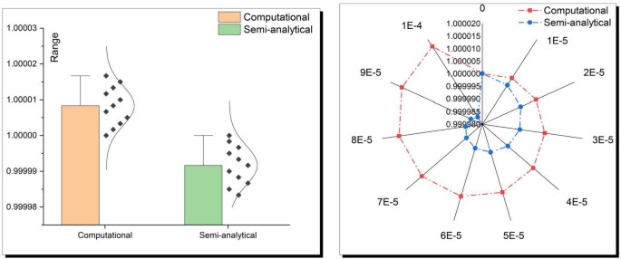
Two-dimensional sketches between the analytical and approximate solutions based on the EK method for illustrating the matching between solutions
Figure 3 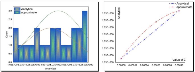
Two-dimensional sketches between the analytical and approximate solutions based on the CBS scheme for illustrating the matching between solutions
Figure 4 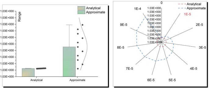
Two-dimensional sketches between the analytical and approximate solutions based on the ECBS method for illustrating the matching between solutions
Figure 5 
Two-dimensional sketches between the analytical and approximate solutions based on the ExCBS method for illustrating the matching between solutions
Figure 6 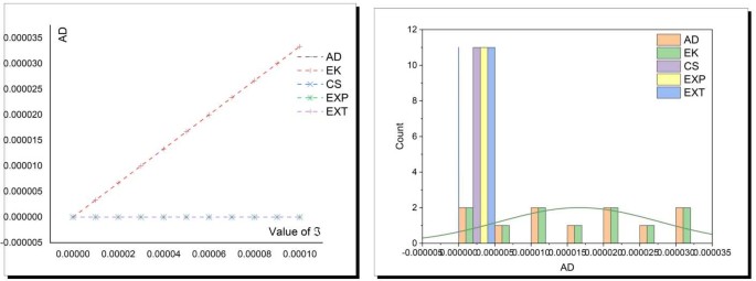
Two-dimensional sketches for the above-used schemes
-
Comparing our obtained numerical results with those obtained in [33], which used the trigonometric quintic B-spline scheme to investigate the numerical solutions of the same model, shows the accuracy of our solutions, which coincide with their solutions, where both of us offer the accuracy of the ESE computational method over other used computational schemes in [1].


4 Conclusion
This manuscript has investigated numerical solutions of the fractional nonlinear telegraph equation by employing five numerical techniques. Abundant numerical results have been obtained, while matching exact and numerical solutions has been explained by some distinct figures in two dimensions. The superiority of the ESE analytical and CBS numerical schemes has been demonstrated. The originality of our paper has been explained by comparing our solutions with previously constructed solutions.
Availability of data and materials
The data that support the findings of this study are available from the corresponding author upon reasonable request.
References
Hamed, Y.S., Khater, M.M.A.: Computational traveling wave solutions of the fractional nonlinear space-time telegraph equation through three recent analytical schemes. J. Math. (2020, in press)
Ellahi, R., Fetecau, C., Sheikholeslami, M.: Recent Advances in the Application of Differential Equations in Mechanical Engineering Problems, Mathematical Problems in Engineering 2018 (2018)
Hosseini, K., Mayeli, P., Ansari, R.: Modified Kudryashov method for solving the conformable time-fractional Klein–Gordon equations with quadratic and cubic nonlinearities. Optik 130, 737–742 (2017)
Delkhosh, M., Parand, K.: A hybrid numerical method to solve nonlinear parabolic partial differential equations of time-arbitrary order. Comput. Appl. Math. 38(2), 76 (2019)
Khater, M.M., Seadawy, A.R., Lu, D.: Dispersive optical soliton solutions for higher order nonlinear Sasa–Satsuma equation in mono mode fibers via new auxiliary equation method. Superlattices Microstruct. 113, 346–358 (2018)
Abdou, M.A.: An analytical method for space–time fractional nonlinear differential equations arising in plasma physics. J. Ocean Eng. Sci. 2(4), 288–292 (2017)
Hosseini, K., Mayeli, P., Ansari, R.: Modified Kudryashov method for solving the conformable time-fractional Klein–Gordon equations with quadratic and cubic nonlinearities. Optik 130, 737–742 (2017)
Guy, T.T., Bogning, J.R.: Modeling nonlinear partial differential equations and construction of solitary wave solutions in an inductive electrical line. J. Adv. Math. Comput. Sci. 1–10 (2019)
Zhang, X., Sagiya, T.: Shear strain concentration mechanism in the lower crust below an intraplate strike-slip fault based on rheological laws of rocks. Earth Planets Space 69(1), 82 (2017)
Pels, A., Gyselinck, J., Sabariego, R.V., Schöps, S.: Solving nonlinear circuits with pulsed excitation by multirate partial differential equations. IEEE Trans. Magn. 54(3), 1–4 (2017)
Cevikel, A.C.: New exact solutions of the space-time fractional KdV-Burgers and nonlinear fractional foam Drainage equation. Therm. Sci. 22(Suppl. 1), 15–24 (2018)
Raissi, M.: Deep hidden physics models: deep learning of nonlinear partial differential equations. J. Mach. Learn. Res. 19(1), 932–955 (2018)
Alabau-Boussouira, F., Ancona, F., Porretta, A., Sinestrari, C.: Trends in Control Theory and Partial Differential Equations, vol. 32. Springer, Berlin (2019)
Lin, H.: Electronic structure from equivalent differential equations of Hartree–Fock equations. Chin. Phys. B 28(8), 087101 (2019)
Ahmad, H., Khan, T.A., Ahmad, I., Stanimirović, P.S., Chu, Y.-M.: A new analyzing technique for nonlinear time fractional Cauchy reaction-diffusion model equations. Results Phys. 2020, 103462 (2020)
Ahmad, H., Akgül, A., Khan, T.A., Stanimirović, P.S., Chu, Y.-M.: New perspective on the conventional solutions of the nonlinear time-fractional partial differential equations. Complexity 2020 (2020)
Ahmad, H., Khan, T.A., Stanimirović, P.S., Chu, Y.-M., Ahmad, I.: Modified variational iteration algorithm-II: convergence and applications to diffusion models. Complexity 2020 (2020)
Abouelregal, A.E., Yao, S.-W., Ahmad, H.: Analysis of a functionally graded thermopiezoelectric finite rod excited by a moving heat source. Results Phys. 19, 103389 (2020)
Attia, R.A., Lu, D., Ak, T., Khater, M.M.: Optical wave solutions of the higher-order nonlinear Schrödinger equation with the non-Kerr nonlinear term via modified Khater method. Mod. Phys. Lett. B 34(05), 2050044 (2020)
Ali, A.T., Khater, M.M., Attia, R.A., Abdel-Aty, A.-H., Lu, D.: Abundant numerical and analytical solutions of the generalized formula of Hirota–Satsuma coupled KdV system. Chaos Solitons Fractals 131, 109473 (2020)
Khater, M.M., Attia, R.A., Abdel-Aty, A.-H., Abdou, M., Eleuch, H., Lu, D.: Analytical and semi-analytical ample solutions of the higher-order nonlinear Schrödinger equation with the non-Kerr nonlinear term. Results Phys. 16, 103000 (2020)
Khater, M.M., Park, C., Abdel-Aty, A.-H., Attia, R.A., Lu, D.: On new computational and numerical solutions of the modified Zakharov–Kuznetsov equation arising in electrical engineering. Alex. Eng. J. (2020)
Khater, M.M., Alzaidi, J., Attia, R.A., Lu, D., et al.: Analytical and numerical solutions for the current and voltage model on an electrical transmission line with time and distance. Phys. Scr. 95(5), 055206 (2020)
Khater, M.M., Attia, R.A., Baleanu, D.: Abundant new solutions of the transmission of nerve impulses of an excitable system. Eur. Phys. J. Plus 135(2), 1–12 (2020)
Li, J., Attia, R.A., Khater, M.M., Lu, D.: The new structure of analytical and semi-analytical solutions of the longitudinal plasma wave equation in a magneto-electro-elastic circular rod. Mod. Phys. Lett. B 2020, 2050123 (2020)
Yue, C., Khater, M.M., Attia, R.A., Lu, D.: The plethora of explicit solutions of the fractional KS equation through liquid–gas bubbles mix under the thermodynamic conditions via Atangana–Baleanu derivative operator. Adv. Differ. Equ. 2020(1), 1 (2020)
Park, C., Khater, M.M., Attia, R.A., Alharbi, W., Alodhaibi, S.S.: An explicit plethora of solution for the fractional nonlinear model of the low–pass electrical transmission lines via Atangana–Baleanu derivative operator. Alex. Eng. J. (2020)
Khater, M.M., Park, C., Lu, D., Attia, R.A.: Analytical, semi-analytical, and numerical solutions for the Cahn–Allen equation. Adv. Differ. Equ. 2020(1), 1 (2020)
Goldstein, S.: On diffusion by discontinuous movements, and on the telegraph equation. Q. J. Mech. Appl. Math. 4(2), 129–156 (1951)
Chen, J., Liu, F., Anh, V.: Analytical solution for the time-fractional telegraph equation by the method of separating variables. J. Math. Anal. Appl. 338(2), 1364–1377 (2008)
Kumar, S.: A new analytical modelling for fractional telegraph equation via Laplace transform. Appl. Math. Model. 38(13), 3154–3163 (2014)
Orsingher, E., Zhao, X.: The space-fractional telegraph equation and the related fractional telegraph process. Chin. Ann. Math. 24(1) (2003)
Khater, M.M., Nisar, K.S., Mohamed, M.S.: Numerical investigation for the fractional nonlinear space-time telegraph equation via the trigonometric quintic B-spline scheme. Math. Methods Appl. Sci. (2020)
Acknowledgements
The authors are thankful to the Taif University. Taif University researchers are supported by project number (TURSP-2020/160), Taif University, Taif, Saudi Arabia.
Funding
This paper was funded by “Taif University Researchers Supporting Project number (TURSP-2020/160), Taif University, Taif, Saudi Arabia”.
Author information
Authors and Affiliations
Contributions
The authors conceived of the study, participated in its design and coordination, drafted the manuscript, participated in the sequence alignment, and read and approved the final manuscript.
Corresponding authors
Ethics declarations
Competing interests
The authors declare that they have no competing interests.
Rights and permissions
Open Access This article is licensed under a Creative Commons Attribution 4.0 International License, which permits use, sharing, adaptation, distribution and reproduction in any medium or format, as long as you give appropriate credit to the original author(s) and the source, provide a link to the Creative Commons licence, and indicate if changes were made. The images or other third party material in this article are included in the article’s Creative Commons licence, unless indicated otherwise in a credit line to the material. If material is not included in the article’s Creative Commons licence and your intended use is not permitted by statutory regulation or exceeds the permitted use, you will need to obtain permission directly from the copyright holder. To view a copy of this licence, visit http://creativecommons.org/licenses/by/4.0/.
About this article

Cite this article
Khater, M.M.A., Park, C., Lee, J.R. et al. Five semi analytical and numerical simulations for the fractional nonlinear space-time telegraph equation. Adv Differ Equ 2021, 227 (2021). https://doi.org/10.1186/s13662-021-03387-9
Received:
Accepted:
Published:
DOI: https://doi.org/10.1186/s13662-021-03387-9