- Research
- Open access
- Published:
On pairs of fuzzy dominated mappings and applications
Advances in Difference Equations volume 2021, Article number: 417 (2021)
Abstract
The main purpose of this paper is to present some fixed-point results for a pair of fuzzy dominated mappings which are generalized V-contractions in modular-like metric spaces. Some theorems using a partial order are discussed and also some useful results to graphic contractions for fuzzy-graph dominated mappings are developed. To explain the validity of our results, 2D and 3D graphs have been constructed. Also, applications are provided to show the novelty of our obtained results and their usage in engineering and computer science.
1 Introduction and preliminaries
The fixed-point theory becomes essential in analysis (see [1–66]). In [19], Chistyakov firstly introduced the notion of a modular metric and discussed thoroughly its convergence, convexity, relation with metrics, convex cones, and the structure of semigroups on such spaces. The modular metric spaces generalize classical modulars over linear spaces, like Orlicz, Lebesgue, Musielak–Orlicz, Lorentz, Calderon–Lozanovskii, and Orlicz–Lorentz spaces. The main idea behind this new concept is the physical interpretation of the modular. We look at these spaces as the nonlinear version of the classical modular spaces. Padcharoen [42] initiated the idea of rational type F-contractions in modular metric spaces and proved some important results. Additional results in such spaces proved by different authors can be seen in [18, 31, 33, 37]. Nadler [39] presented a fixed-point theorem for multivalued mappings and generalized its analogues for single-valued mappings. Fixed-point results of multivalued mappings have several applications in engineering, control theory, differential equations, games and economics; see [11, 16]. In this paper, we are using multivalued mappings. Wardowski [66] introduced a new type of contractions, named F-contractions, to obtain a fixed-point result. For more results in this direction, see [2, 3, 6, 8, 15, 32, 33, 38, 55]. Here, we have used a weak family of mappings instead of the function F introduced by Wardowski. In [9] the authors observed that there are mappings which possess fixed points. Namely, they introduced a condition on closed balls to achieve common fixed points for such mappings. For further results on closed balls, see [50, 51, 63]. In this paper, we are using a sequence instead of a closed ball. Ran and Reurings [49] and Nieto and Rodríguez-López [41] gave fixed-point theory results in partially ordered sets. For more results in ordered spaces, see [20, 21, 23]. Asl et al. [10] gave the notion of \(\alpha _{*}\)-admissible mappings and α–ω-contractive set-valued mappings (see also [5, 26, 29, 56]) and generalized the restriction of order. Rasham et al. [53] introduced the concept of \(\alpha _{*}\)-dominated mappings to establish a new condition of order and obtained some results (see also [52, 54, 59, 62]). They proved that there are mappings which are \(\alpha _{*}\)-dominated, but not \(\alpha _{*}\)-admissible. The notion of fuzzy sets is introduced by Zadeh [67] and then a lot of researchers did their research work in this field. Weiss [68] and Butnariu [17] firstly discussed the concept of fuzzy mappings and showed many related results. Heilpern [16] discussed a result on fuzzy mappings, which was a further generalization of Nadler’s set-valued result [39] using a Hausdorff metric. Due to importance of the Heilpern’s results, fixed-point theory for fuzzy contractions using a Hausdorff metric has become more important, see [44–48, 51, 61, 62]. In this article, we prove fixed point results for a pair of fuzzy dominated maps which are generalized V-contractions and provide related graphs for 2D and 3D. An application for the solution of electric circuit equations is also presented. Moreover, a fractional differential equation is solved. Our obtained results generalize those presented in [54, 57, 59, 61, 66].
We start with the following statements which are helpful to prove our results.
Definition 1.1
([56])
Let A be a nonempty set. A function \(u: (0,1) \times A \times A \rightarrow [0,1)\) is called a modular-like metric on A if for all \(a,b,c \in A; l,n> 0\), and \(u_{l} (a,b) = u(l,a,b)\), the following hold:
-
(i)
\(u_{l} ( a, b ) = u_{l} ( b, a )\);
-
(ii)
\(u_{l} ( a, b ) = 0\), then \(a = b\);
-
(iii)
\(u_{l + n} ( a, b )\leq u_{l} ( a, c ) + u_{n} ( c, b )\).
\({ (A, u)}\) is called a modular-like metric space. If we replace (ii) by \(u_{l} ( a, b ) = 0\) if and only if \(a = b\), then (\(A, u\)) becomes a modular metric space. If we replace (ii) by \(u_{l} (a, b) = 0\) for some \(l > 0\) then \(a = b\), then \((A; u)\) becomes a regular modular-like metric on A. For \(e \in A\) and \(\epsilon > 0, B_{u_{l}} (e,\epsilon )= \{ p\in A: \vert u_{l} ( e,p ) - u_{l} ( e,e ) \vert \leq \epsilon ) \}\) is the closed ball. We abbreviate by “\(m.l.m\). space” a modular-like metric space.
Definition 1.2
([56])
Let (\(A, u\)) be an \(m.l.m\). space.
-
(i)
A sequence \((a_{n} )_{n\in \mathbb{N}}\) in A is u-Cauchy for some \(l > 0\), if and only if \(\lim_{n,m\rightarrow +\infty } u_{l} ( a_{m}, a_{n} )\) exists and is finite.
-
(ii)
A sequence \((a_{n} )_{n\in \mathbb{N}}\) in A u-converges to \(a \in A\) for some \(l > 0\), if and only if \(\lim_{n\rightarrow +\infty } u_{l} ( a_{n},a ) = u_{l} ( a,a ) \).
-
(iii)
\(E\subseteq A\) is called u-complete if any u-Cauchy sequence \(\{ a_{n} \} \) in E is u-convergent to some \(a\in E\), so that for some \(l>0\),
Definition 1.3
([57])
Let (\(A, u\)) be an \(m.l.m\). space and \(E\subseteq A\). An element \(p_{0}\) of A is the closest to E if it provides the finest estimate in E for \(e \in A\), i.e.,
If every \(e \in A\) has a greatest estimate in E, then E is identified as a proximal set. For example, let \(A = \mathbb{R}^{+} \cup \{0\}\) and \(u_{l} (e, p) = \frac{1}{l} (e + p)\) for all \(l > 0\). Define a set \(E = [ 4, 6 ]\), then for each \(y \in A\),
Hence, 4 is the finest estimate in E for very \(y \in A\). Also, [\(4, 6\)] is a proximal set.
From now on, denote by \(P (A)\) the set of compact proximinal subsets in A.
Definition 1.4
([56])
Let \((A, u)\) be an \(m.l.m\). space. The function \(_{H u_{l}}:P (A)\times P (A) \rightarrow [0, \infty)\), given as
is \(u_{l}\)-Hausdorff metric like. The pair (\(P ( A ), H_{u_{l}} \)) is named as a \(u_{l}\)-Hausdorff metric like space.
For examples, take \(A= R^{+} \cup \{0\}\). Let
If \(N= [ 3,5 ], R= [ 7,8 ]\), then \(H_{u_{l}} ( N,R ) = \frac{13}{l} \).
Definition 1.5
([56])
Let (\(A,u\)) be an \(\mathit{m.l.m.}\) space. We will say that u satisfies the \(\Delta _{M}\)-condition if \(\lim_{n,m\rightarrow \infty } u_{p} ( e_{n}, e_{m} ) =0\), where \(p\in \mathbb{N}\) implies \(\lim_{n,m\rightarrow \infty } u_{l} ( e_{n}, e_{m} ) =0 \), for some \(l>0\).
Definition 1.6
([62])
Let A be a nonempty set, \(G:A\rightarrow P(A)\), \(B\subseteq A\), and \(\alpha:A\times A\rightarrow [ 0,+\infty ) \). Then G is said to be \(\alpha _{*}\)-admissible on B if
whenever \(\alpha ( p,c ) \geq 1\), for all \(p,c\in B\).
Definition 1.7
([53])
Let A be a nonempty set, \(G:A\longrightarrow P ( A )\), \(M\subseteq A\), and \(\alpha:A\times A\rightarrow [ 0, +\infty ) \). Then G is named as \(\alpha _{*}\)-dominated on M, if for any \(b\in M \),
Example 1.8
([53])
Let \(B= ( -\infty,\infty ) \). Define \(\gamma:B\times B\rightarrow [0, \infty)\) and \(K,L:B\rightarrow P ( B )\), respectively, by
and
Then K and L are not \(\gamma _{*}\)-admissible, but they are \(\gamma _{*}\)-dominated.
Definition 1.9
([66])
Consider a metric space \(( M,d ) \). A mapping \(G:M\rightarrow M\) is called an F-contraction if for all \(b,c\in M,\exists \tau >0\) such that \(d(Gb,Gc)>0\) we have
where \(F: \mathbb{R}_{+} \rightarrow\mathbb{ R}\) is such that:
(F1) There is \(k\in (0,1)\) such that \(\lim_{\sigma \rightarrow 0^{+}} \sigma ^{k} F ( \sigma ) =0\);
(F2) F is strictly increasing;
(F3) \(\lim_{n\rightarrow +\infty } \sigma _{n} =0\) if \(\lim_{n\rightarrow +\infty } F ( \sigma _{n} ) =-\infty \), for each sequence \(\{ \sigma _{n} \} _{n=1}^{\infty } \) of positive numbers.
The family of functions verifying (F1)–(F3) is denoted by R.
Lemma 1.10
Let \(( Q,u )\) be an \(\mathit{m.l.m.}\) space. Let \(( P ( Q ), H_{u_{1}} )\) be a \(u_{1}\)-Hausdorff metric like space. Then, for any \(e\in C\) and for all \(C,D\in P ( Q )\), there is \(y_{e} \in D\) such that
Definition 1.11
([60])
A fuzzy set U is a function from G to \([0,1]\) and \(F(G)\) is the family of all fuzzy sets in G. If U is a fuzzy set and \(e\in G\), then \(U(e)\) is said to be the grade of membership of e in U. The β-level set of the fuzzy set U is denoted by \([U]_{\beta }\), and is given as
Now, we select a subset of the family \(F(G)\) of all fuzzy sets, which is a subfamily with stronger properties, i.e., the subfamily of the approximate quantities, denoted by \(W(G)\).
Definition 1.12
([24])
A fuzzy subset U of G is an approximate quantity iff its β-level set is a compact convex subset of G for each \(\beta \in [ 0,1 ]\) and \(\sup_{e\in G} U ( e ) =1\).
Definition 1.13
([24])
Let R be an arbitrary set and G be any metric space. A fuzzy map is a mapping from R to \(W ( G ) \). We can view a fuzzy mapping \(T:R\rightarrow W(G)\) as a fuzzy subset of \(R\times G, T:R\times G\rightarrow [ 0,1 ]\) in the sense that \(T ( c,y ) =T ( c ) ( y ) \).
Definition 1.14
([60])
A point \(c\in M\) is called a fuzzy fixed point of a fuzzy mapping \(T:M\rightarrow W(M)\) if there exists \(0<\beta \leq 1\) such that \(c\in [Tc]_{\beta } \).
Definition 1.15
Let A be a nonempty set, \(\xi:A\rightarrow W ( A )\) be a fuzzy mapping, \(M\subseteq A\), and \(\alpha:A\times A\rightarrow [ 0,+\infty ) \). Then ξ is named as fuzzy \(\alpha _{*}\)-dominated on M, if for each \(a\in M\) and \(0<\beta \leq 1 \),
Now, we are ready to prove our main theorems for a pair of fuzzy mappings which are a generalized rational type contraction.
2 Main results
Let \(( \mathcal{L}, u )\) be an \(\mathit{m.l.m.}\) space, \(x_{0} \in \mathcal{L}\) and \(S,T:\mathcal{L}\rightarrow W ( \mathcal{L} )\) be fuzzy mappings on \(\mathcal{L}\). Moreover, let \(\gamma,\beta: \mathcal{L}\rightarrow [ 0;1 ]\) be two real functions. Let \(x_{1} \in S [ x_{0} ]_{\gamma ( x_{0} )}\) be an element such that \(u_{1} ( x_{0}, [ S x_{0} ]_{\gamma ( x_{0} )} ) = u_{1} ( x_{0}, x_{1} ) \). Let \(x_{2} \in [ T x_{1} ]_{\beta ( x_{1} )}\) be such that \(u_{1} ( x_{1}, [ T x_{1} ]_{\beta ( x_{1} )} ) = u_{1} ( x_{1}, x_{2} )\). Let \(x_{3} \in [ S x_{2} ]_{\gamma ( x_{2} )}\) be such that \(u_{1} ( x_{2}, [ S x_{2} ]_{\gamma ( x_{2} )} ) = u_{1} ( x_{2}, x_{3} ) \). Continuing this process, we construct a sequence \(\{ x_{n} \}\) of points in \(\mathcal{L}\) such that
Also,
We use \(\{ TS ( x_{n} ) \} \) to denote this sequence. We say that \(\{TS( x_{n} )\}\) is a sequence in \(\mathcal{L}\) generated by \(x_{0}\).
Definition 2.1
Let (\(\mathcal{L}, u\)) be a complete \(\mathit{m.l.m.}\) space. Suppose that u is regular and the \(\Delta _{M}\)-condition holds. Let \(x_{0} \in \mathcal{L}, \alpha: \mathcal{L}\times \mathcal{L}\rightarrow [ 0,\infty)\) and \(S,T:\mathcal{L}\rightarrow W (\mathcal{L})\) be two fuzzy \(\alpha _{*}\)-dominated mappings on \(\{TS ( x_{n} ) \}\). The pair (\(S,T\)) is called a rational fuzzy dominated V-contraction if there exist \(\tau >0, \gamma ( x ), \beta ( x ) \in ( 0,1 ]\) and \(V\in R\) such that
whenever, \(x,g\in \{ TS ( x_{n} ) \}, \alpha ( x,g ) \geq 1, \text{ and } H_{u_{1}} ( [ Sx ]_{\gamma ( x )}, [ Tg ]_{\beta ( g )} )>0\).
Theorem 2.2
Let (\(\mathcal{L}, u\)) be a complete \(\mathit{m.l.m.}\) space. Assume that \(S,T:\mathcal{L}\rightarrow W (\mathcal{L})\) are two fuzzy \(\alpha _{*}\)-dominated mappings on \(\{ TS ( x_{n} ) \} \). If (\(S,T\)) is a rational fuzzy dominated V-contraction, then \(\{TS( x_{n} )\}\) is a Cauchy sequence in \(\mathcal{L}\) and \(\{ TS ( x_{n} ) \} \rightarrow k \in \mathcal{L}\).
Proof
As \(S,T:\mathcal{L}\rightarrow W ( \mathcal{L} )\) are two fuzzy \(\alpha _{*}\)-dominated mappings on \(\{ TS ( x_{n} ) \} \), so, by definition, we have
for all \(i \in \mathbb{N}\). As \(\alpha _{*} ( x_{2i},[ S x_{2i} ]_{\gamma ( x_{2i} )} )\geq 1\), this implies that \(\inf \{\alpha ( x_{2i}, b ): b\in [ S x_{2i} ]_{\gamma ( x_{2i} )} \}\geq 1\) and therefore, \(\alpha ( x_{2i}, x_{2i+1} )\geq 1\). Now, by using Lemma 1.10, we have
This implies that
If \(\max \{ u_{1} ( x_{2i}, x_{2i+1} ), u_{1} ( x_{2i+1}, x_{2i+2} ) \})= u_{1} ( x_{2i+1}, x_{2i+2} )\), then from (2.2), we have
It is a contradiction. Therefore,
Hence, from (2.2), we have
Similarly, we have
For all \(i\in \{ 0,1,2,\dots. \} \). By (2.4) and (2.3), we have
Repeating these steps, we get
Similarly, we have
Inequalities (2.5) and (2.6) can jointly be written as
Taking the limit as \(n\rightarrow \infty \) in (2.7), we have
Since \(V\in R\), one gets
Applying the property \(( F1)\), we have some \(k\in ( 0,1 )\), for which
By (2.7), for all \(n\in \mathbb{N}\), we obtain
Considering (2.8), (2.9) and letting \(n\rightarrow \infty \) in (2.10), we have
Since (2.11) holds, there exists \(n_{1} \in\mathbb{ N}\) such that \(n (u_{1} ( x_{n}, x_{n+1} ))^{k} \leq 1\) for all \(n\geq n_{1}\), or
Take \(p>0\) and \(m=n+p>n> n_{1}\), then
As \(k\in (0,1)\), then \(\frac{1}{k} >1\) and, by the ratio test,
Since u satisfies the \(\Delta _{M}\)- condition, we have
Hence, the sequence \(\{ TS ( x_{n} ) \} \) is Cauchy in the complete regular modular-like type metric space (\(\mathcal{L}, u\)), hence there is \(k \in \mathcal{L}\) so that \(\{ TS ( x_{n} ) \} \rightarrow k \text{ as } n\rightarrow \infty \). □
Theorem 2.3
Let (\(\mathcal{L}, u\)) be a complete \(\mathit{m.l.m.}\) space. Assume that \(S,T:\mathcal{L}\rightarrow W (\mathcal{L})\) are two fuzzy \(\alpha _{*}\)-dominated mappings on \(\{ TS ( x_{n} ) \} \). If (\(S,T\)) is a rational fuzzy dominated V-contraction and k is the limit of the sequence \(\{ TS ( x_{n} ) \} \). If \(\alpha ( x_{n},k ) \geq 1 \forall n\in \{0,1,2,\ldots \}\), then k belongs to both \([ Tk]_{\beta ( k )}\) and \([ Sk]_{\gamma ( k )}\).
Proof
As (\(S, T\)) is a rational fuzzy dominated V-contraction, then, by Theorem 2.2, there exists \(k \in \mathcal{L}\) such that \(\{ TS ( x_{n} ) \} \rightarrow k\) as \(n\rightarrow \infty \) and so
Now, by Lemma 1.10, we have
By supposition, \(\alpha ( x_{n},k ) \geq 1\), so assume that \(u_{1} (k, [ Tk]_{\beta ( k )} )>0\), then there must be a positive natural number p so that \(u_{1} ( x_{2n+1},[ Tk]_{\beta ( k )} )>0\), for every \(n\geq p\). Now, \(H_{u_{1}} ( [ S x_{2n} ] \gamma _{x_{2n}}, [ Tk]_{\beta ( k )} )>0\), so inequality (2.1) implies for every \(n\geq p\),
Letting \(n\rightarrow \infty \) and using (2.15), we get
Since V is strictly increasing, (2.16) implies that
This is a contradiction. So, our supposition is not true. Hence \(u_{1} (k,[ Tk]_{\beta ( k )} )=0\) or \(k\in [ Tk]_{\beta ( k )} \). Similarly, by proceeding Lemma 1.10 and inequality (2.1), we can prove that
Hence, S and T have a common fuzzy fixed point k in \(\mathcal{L}\). □
Definition 2.4
Let \(\mathcal{L}\) be a nonempty set, ≼ be a partial order on \(B \subseteq \mathcal{L}\). We say that \(a\preccurlyeq B\) whenever for all \(b\in B\), we have \(a\preccurlyeq b\). A mapping \(S:\mathcal{L}\rightarrow W (\mathcal{L})\) is said to be fuzzy ≼-dominated on B, if \(a\preccurlyeq [Sa ]_{\gamma } \) for each \(a \in \mathcal{L} and \gamma \in ( 0,1 ] \).
We have the following result for multi fuzzy ≼-dominated mappings on \(\{TS ( x_{n} ) \}\) in an ordered complete \(\mathit{m.l.m.}\) space.
Theorem 2.5
Let (\(\mathcal{L},\preccurlyeq, u\)) be an ordered complete \(\mathit{m.l.m.}\) space. Suppose that u is regular and the \(\Delta _{M}\)-condition holds. Take \(x_{0} \in \mathcal{L}\) and let \(S,T:\mathcal{L}\rightarrow W (\mathcal{L})\) be fuzzy dominated mappings on \(\{TS ( x_{n} ) \}\). Suppose there exist \(\tau >0,\gamma ( x ),\beta ( g ) \in (0,1]\) and \(V\in R\) such that the following holds:
whenever \(x,g\in \{ TS ( x_{n} ) \}\), with either \(x\preccurlyeq g\) or \(g\preccurlyeq x\), and \(H_{u_{1}} ( [ Sx ]_{\gamma (x)},[ Tg]_{\beta ( g )} )>0\). Then \(\{ TS ( x_{n} ) \} \rightarrow k \in \mathcal{L}\). Also, if (2.17) holds for k, \(x_{n} \preccurlyeq k\) and \(k\preccurlyeq x_{n}\) for all \(n\in \{ 0,1,2,\ldots \} \), then k belongs to both \([ Tk]_{\beta ( k )}\) and \([Sk]_{\gamma ( k )} \).
Proof
Let \(\alpha:\mathcal{L}\times \mathcal{L}\rightarrow [ 0,+\infty)\) be a mapping defined by \(\alpha ( x,g ) =1\) for all \(x \in \mathcal{L}\) with \(x\preccurlyeq g\), and \(\alpha ( x,g ) =0\) for all other elements \(x,g \in \mathcal{L}\). As S and T are the fuzzy prevalent mappings on \(\mathcal{L}\), so \(x\preccurlyeq [ Sx]_{\gamma ( x )}\) and \(x\preccurlyeq [ Tx]_{\beta ( x )}\) for all \(x \in \mathcal{L}\). This implies that \(x\preccurlyeq b\) for all \(b\in [ Sx]_{\gamma ( x )}\) and \(x \preccurlyeq e\) for all \(x\in [ Tx]_{\beta ( x )}\). So, \(\alpha ( x,b ) =1\) for all \(b\in [ Sx]_{\gamma ( x )}\) and \(\alpha ( x,e ) =1\) for all \(x\in [ Tx]_{\beta ( x )}\). This implies that
Hence, \(\alpha _{*} (x, [ Sx]_{\gamma ( x )} )=1, \alpha _{*} (x, [ Tx]_{\beta ( x )} )=1\) for all \(x \in \mathcal{L}\). So, \(S,T:\mathcal{L}\rightarrow W (\mathcal{L} )\) are \(\alpha _{*}\)-dominated mappings on \(\mathcal{L}\). Moreover, inequality (2.17) holds and it can be written as
for all elements \(x,g\) in \(\{TS ( x_{n} ) \}\), with either \(\alpha ( x,g ) \geq 1\) or \(\alpha ( g,x ) \geq 1\). Then, by Theorem 2.2, \(\{ TS ( x_{n} ) \}\) is a sequence in \(\mathcal{L}\) and \(\{TS ( x_{n} ) \}\rightarrow x^{*} \in \mathcal{L}\). Now, \(x_{n}, x^{*} \in \mathcal{L}\) and either \(x_{n} \preccurlyeq x^{*}\), or \(x^{*} \preccurlyeq x_{n}\) implies that either \(\alpha ( x_{n}, x^{*} )\), or \(\alpha ( x^{*}, x_{n} )\geq 1\). So, all requirements of Theorem 2.3 are satisfied. Hence, \(x^{*}\) is the common fuzzy fixed point of both S and T in \(\mathcal{L}\) and \(u_{l} ( x^{*}, x^{*} ) =0\). □
Example 2.6
Let \(\mathcal{L}= Q^{+} \cup \{0\}\) and \(u_{l} ( e,x ) = \frac{1}{l} ( e+x ) \). Now,
\(\forall e, x \in \mathcal{L}\). Define \(S, T:\mathcal{L}\longrightarrow W ( \mathcal{L} )\) by
Now, we consider
Taking \(e_{0} = \frac{1}{2}\), then we have
So, we obtain a sequence \(\{ TS ( e_{n} ) \} = \{ \frac{1}{2}, \frac{1}{8}, \frac{1}{24}, \frac{1}{96},\dots. \} \) in \(\mathcal{L}\) generated by \(e_{0} \).
Now, for all \(e,x\in \{TS ( c_{n} ) \}\) with either \(\alpha ( e, x ) \geq 1 \text{ or } \alpha (x, e)\geq 1\), we have
-
i.
Case (1): If \(\max \{ ( \frac{3e}{4} + \frac{x}{3} ), ( \frac{e}{4} + \frac{2x}{3} ) \} =( \frac{3e}{4} + \frac{x}{3} )\) and \(\tau = \ln ( 1.2 )\), then we have
$$\begin{aligned} \frac{9e}{2} +2x\leq 5e+5x. \end{aligned}$$Then
$$\begin{aligned} \frac{6}{5} \biggl( \frac{3e}{4} + \frac{x}{3} \biggr) \leq e+x. \end{aligned}$$Therefore,
$$\begin{aligned} \ln (1.2) + \ln \biggl( \frac{3e}{4} + \frac{x}{3} \biggr)\leq \ln ( e+x ). \end{aligned}$$This implies that
Figure 1 illustrates Case (i) of Example 2.6, where the graph in blue represents the right side of the contractive inequality of Theorem 2.3 and that in red shows the left side of the inequality of Theorem 2.3.
Figure 1 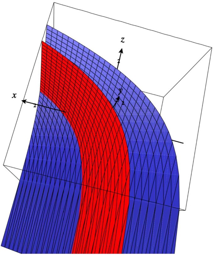
Comparison of the functions \(V ( H_{u_{1}} ( [ Se ]_{\frac{\gamma }{2}}, [ T x ]_{\frac{\beta }{4}} ) )\) and \(E ( N ( e, x ) )\).
 ;
; 
-
ii.
Case (ii): If \(\max \{ ( \frac{3e}{4} + \frac{x}{3} ), ( \frac{e}{4}, \frac{2x}{3} ) \} =( \frac{e}{4} + \frac{2x}{3} )\) and \(\tau = \ln ( 1.2 )\), then we have
$$\begin{aligned} \frac{3e}{2} +4x\leq 5e+5x. \end{aligned}$$That is,
$$\begin{aligned} \frac{6}{5} \biggl( \frac{e}{4} + \frac{2x}{3} \biggr) \leq e+x. \end{aligned}$$Then
$$\begin{aligned} \ln (1.2) + \ln \biggl( \frac{e}{4} + \frac{2x}{3} \biggr)\leq \ln ( e+x ). \end{aligned}$$This implies that

 ;
; 
Figure 2 illustrates Case (ii) of Example 2.6, where the graph in blue represents the right side of the contractive inequality of Theorem 2.3 and that in red shows the left side of the inequality of Theorem 2.3 (See Figure 3).

Comparison of the functions \(E ( H_{u_{1}} ( [ Se ]_{\frac{\gamma }{2}}, [ T x ]_{\frac{\beta }{4}} ) )\) and \(E ( N ( e, x ) )\).  ;
; 

Graph for lnx. 
Hence, all requirements of Theorem 2.3 are satisfied.
Corollary 2.7
Let (\(\mathcal{L}, u\)) be a complete \(\mathit{m.l.m.}\) space. Assume that u is regular and the \(\Delta _{M}\)-condition holds. Take \(x_{0} \in \mathcal{L}, \alpha:\mathcal{L}\times \mathcal{L}\longrightarrow [0,\infty)\) and let \(S:\mathcal{L}\longrightarrow W (\mathcal{L})\) be a fuzzy \(\alpha _{*}\)-dominated mapping on \(\{ SS( x_{n} ) \} \). Suppose there exist \(\tau >0,\gamma ( x ), \beta ( g ) \in ( 0,1 ]\), and \(V\in R\) such that
whenever \(x,g\in \{ SS ( x_{n} ) \},\alpha (x,g)\geq 1\) and \(H_{u_{1}} ( [Sx]_{\gamma (x)}, [Sg]_{\beta (g)} ) >0\). Then \(\alpha ( x_{n}, x_{n+1} ) \geq 1\) for all \(n\in \{0,1,2,\dots \}\) and \(\{ SS( x_{n} ) \} \rightarrow k \in \mathcal{L}\). Also, if either \(\alpha ( x_{n},k)\geq 1\) or \(\alpha (k, x_{n} )\geq 1\) for all \(n\in \{ 0,1,2\dots \} \), then \(k\in [ Sk ]_{\gamma ( k )} \).
If we take multivalued \(\alpha _{*}\)-dominated mappings from a ground set \(\mathcal{L}\) to the proximinal subsets of \(\mathcal{L}\) instead of fuzzy \(\alpha _{*}\)-dominated mappings from \(\mathcal{L}\) to the approximate quantities \(W ( \mathcal{L} )\) in Theorem 2.3, we obtain the following result.
Corollary 2.8
Let (\(\mathcal{L}, u\)) be a complete modular-like metric space. Assume that u is regular and verifies the \(\Delta _{M-}\) condition. Let \(x_{0} \in \mathcal{L}, \alpha:\mathcal{L}\times \mathcal{L}\rightarrow [ 0,\infty)\) and \(S, T: \mathcal{L}\rightarrow W (\mathcal{L})\) be two \(\alpha _{*}\)-dominated mappings on \(\{ TS( x_{n} ) \} \). Suppose there exist \(\tau >0\) and \(V\in R\) such that
whenever \(x,g\in \{ TS ( x_{n} ) \},\alpha (x,g)\geq 1\), and \(H_{u_{1}} (Sx,xg)>0\). Then, \(\alpha ( x_{n}, x_{n+1} )\geq 1\) for all \(n\in \{0,1,2,\dots \}\) and \(\{ TS( x_{n} ) \} \rightarrow k \in \mathcal{L}\). Also, if either \(\alpha ( x_{n},k)\geq 1\) or \(\alpha (k, x_{n} )\geq 1\) for all \(n\in \{ 0,1,2\dots \} \), then k belongs to both Tk and Sk.
If we take \(S=T\) in Corollary 2.8, we obtain the following result.
Corollary 2.9
Let (\(\mathcal{L}, u\)) be a complete modular-like metric space metric space. Assume that u is regular and satisfies the \(\Delta _{M}\)-condition. Let \(x_{0} \in \mathcal{L}, \alpha:\mathcal{L}\times \mathcal{L}\rightarrow [ 0,\infty)\) and \(S: \mathcal{L}\rightarrow W (\mathcal{L})\) be a multivalued \(\alpha _{*}\)-dominated mapping on \(\{ SS( x_{n} ) \} \). Suppose there exist \(\tau >0\) and \(V\in R\) such that
whenever \(x,g\in \{ SS ( x_{n} ) \}, \alpha (x,g)\geq 1\), and \(x_{u_{1}} (Sx,Sg)>0\). Then \(\alpha ( x_{n}, x_{n+1} )\geq 1\) for all \(n\in \{0,1,2,\dots \}\) and \(\{ SS( x_{n} ) \} \rightarrow k \in \mathcal{L}\). Also, if either \(\alpha ( x_{n},k)\geq 1\) or \(\alpha (k, x_{n} )\geq 1\) for all \(n\in \{ 0,1,2,\dots \} \), then k belongs to Sk.
3 Applications on graphic contractions
Jachymski [30] proved a relation between graph and fixed point theory by the orientation of graphic contractions. Let A be a nonempty set. Let \(V(Y )\) and \(L ( Y )\) denote the set of vertices and the set of edges containing all loops, respectively, for a graph Y.
Definition 3.1
Let A be a nonempty set and \(Y= ( V ( Y ),L ( Y ) )\) be a graph with \(A=V ( Y ) \). A fuzzy map F from A to \(W ( A )\) is called fuzzy-graph dominated on A if \(( a,b ) \in L ( Y )\), for \(a\in A\), \(b\in [Fa ]_{\beta } \) and \(0<\beta \leq 1\).
Theorem 3.2
Let \((\mathcal{L}, u)\) be a complete \(\mathit{m.l.m.}\) space equipped with a graph \(Y, x_{0} \in \mathcal{L}\) so that
(i) \(S,T:\mathcal{L}\rightarrow W (\mathcal{L})\) are fuzzy-graph dominated functions on \(\{ TS ( p_{n} ) \} \);
(ii) \(\tau +V( H_{u_{1}} ([St ]_{\gamma ( t )},[Ty ]_{\beta ( y )} ) )\), and \(\tau >0, \gamma ( t ), \beta ( y ) \) in [\(0,1\)]
whenever \(t,y\in \{TS\}( \boldsymbol{x}_{\boldsymbol{n}} )\}, ( t,y)\in L(Y), \textit{ and } H_{u1} ([St ]_{\gamma ( t )}, [ Ty ]_{\beta ( y )} ) >0\). Suppose that \(\mathcal{L}\) is regular and the \(\triangle _{M}\)-condition holds. Then (\(x_{n,} x_{n+1} )\in L(Y)\) and \(\{ TS( x_{n} )\}\rightarrow k^{*}\). Also, if (\(x_{n}, k^{*} )\in L(Y\)) or (\(k^{*}, x_{n} )\in L(Y\)) for each \(n\in \{ 0,1,2,\dots \}, \textit{ then } k^{*}\) belongs to both \([T k^{*} ]_{\beta ( k^{*} )}\) and \(k\in [S k^{*} ]_{\gamma ( k^{*} )} \).
Proof
Define \(\alpha:\mathcal{L}\times \mathcal{L}\rightarrow [ 0,\infty)\) by \(\alpha ( t,y ) =1\), if \(t \in \mathcal{L}\) and \(( t,y ) \in L ( Y ) \). Otherwise, take \(\alpha ( t,y ) =0\). The graph dominated notion on \(\mathcal{L}\) gives that \((t,y )\in L(Y)\) for all \(y\in [St ]_{\gamma ( t )}\) and \((t,y )\in L(Y)\) for each \(y\in [Ty ]_{\beta (y)}\). So, \(\alpha ( t,y ) =1\) for all \(y\in [St ]_{\gamma ( t )}\) and \(\alpha ( t,y ) =1\) for every \(y \in [Ty ]_{\beta (y)}\). This means that
Hence, \(\alpha _{*} (t,[St ]_{\gamma ( t )} )=1, \alpha _{*} (t,[Ty ]_{\beta ( y )} )=1\), for every \(t \in \mathcal{L} \). So, the mappings are \(\alpha _{*} \)-dominated on \(\mathcal{L}\). Furthermore, inequality (3.1) can be expressed as
whenever \(t,y \in \{ TS ( x_{n} ) \}, \alpha (t,y)\geq 1\) and \(H_{u_{1}} ([St ]_{\gamma ( t )}, [Ty ]_{\beta ( y )} )>0\). Also, (ii) holds. Using Theorem 2.2, we have \(\{TS ( x_{n} ) \}\) is a sequence in \(\mathcal{L}\) and \(\{ TS ( x_{n} ) \} \rightarrow k^{*} \in \mathcal{L}\). Now, \(x_{n}, k^{*} \in \mathcal{L}\) and either \(( x_{n}, k^{*} ) \in L ( Y )\), or \(( k^{*}, x_{n} ) \in L(Y)\) implies that either \(\alpha ( x_{n}, k^{*} ) \geq 1 \text{ or } \alpha ( k^{*}, x_{n} )\geq 1\). So,all conditions of Theorem 2.2 are checked. Hence, \(k^{*}\) belongs to both \([T k^{*} ]_{\beta ( k^{*} )}\) and \(k\in [S k^{*} ]_{\gamma ( k^{*} ).}\) □
4 Applications to electric circuit equations
In this section, we discuss the solution of the electric circuit equation (see [7]) which is a second-order differential equation. The electric circuit (as in Fig. 4) contains an electromotive force E, a resistor R, an inductor L, a capacitor C, and a voltage V in series. If the current I is the rate of change of q with respect to time t, we have \(I= \frac{dq}{dt}\) and

Electric circuit
By Kirchhoff’s law, the sum of these voltage drops is equal to supplied voltage, i.e.,
or
The Green function associated to (ECE) is given by
where the constant \(\tau >0\) is calculated in terms of R and L. Let \(\mathcal{L} =C[0,1]\) be the set of all continuous functions defined on \([0,1]\). The modular-like metric u on \(\mathcal{L}\) is defined as
Moreover, we define the graph with the partial order relation: for \(u,g\in C [ 0,1 ] \),
for all \(t\in [ 0,1 ] \). Let \(Y ( G ) =\{(u,g)\in \mathcal{L} \times \mathcal{L}:u\leq g\}\). Note that (\(u, \mathcal{L} \)) is a complete modular-like metric space, including a direct graph G; \(\Delta =( \mathcal{L} \times \mathcal{L} )\in Y(G)\) and (\(u, \mathcal{L},G\)) has a property \(( E^{*} ) \).
Theorem 4.1
Let \(S,T:C[0,1]\rightarrow C[0,1]\) be self-mappings of the modular-like metric space \((C [ 0,1 ),u)\). Assume that
-
(i)
There exist continuous and nondecreasing functions \(H,Q:C[0,1]\times \mathbb{R}\rightarrow \mathbb{R}\) such that for all \(b,c\in C [ 0,1 ]\), with \(b\leq c\), there exists \(\tau >0\) so that
$$\begin{aligned} H \bigl( t,b(s) \bigr) +Q\bigl(t,c(s)\bigr)\leq \frac{\tau E(b,c)}{\tau E ( b,c ) +1}, \end{aligned}$$where
for all \(t,s\in [0,1]\) and \(b,c\in C( [ 0,1 ], \mathbb{R}^{+} )\).
-
(ii)
There are \(b_{0}\), \(c_{0} \in C([0,1])\)
$$\begin{aligned} b_{0}(t)\leq \int _{0}^{t} G ( t,s ) H \bigl( t,b_{0} ( s ) \bigr) \,ds \quad\textit{for all } t\in [0,1] \end{aligned}$$and
$$\begin{aligned} c_{0}\leq \int _{0}^{t} G ( t,s ) Q \bigl( t,c_{0} ( s ) \bigr) \,ds \quad\textit{for all } t\in [ 0,1 ]. \end{aligned}$$Then the differential equation arising in the electric circuit (ECE) has a solution.
Proof
The problem (ECE) is equivalent to integral forms given as
and
where \(t\in [ 0,1 ] \). Consider \(S,T: \mathcal{L} \rightarrow \mathcal{L}\) defined by
and
where \(t\in C[0,1]\). Then \(b^{*}\) is the solution of (4.1) and (4.2) if and only if \(b^{*}\) is a common fixed point of S and T. From condition (ii), it is very easy to show that for every \(u,g\in \mathcal{L}\), we have \(u\leq Su\) and \(g\leq Tg\), i.e.,
Let \(b,g\in \mathcal{L}\), then from condition (i), we have
This implies that
Since \(1-2tr+t\tau e^{-\tau t} - e^{-\tau t} \leq 1\), we get that
which further implies
So, all the requirements of Theorem 2.2 are satisfied for \(R ( f ) = \frac{-1}{f},f>0\), and \(u ( b,c ) = \frac{1}{2} \Vert b+c \Vert _{\tau } \). Hence, the mappings S and T have a common fixed point. Consequently, the differential equation arising in the electric circuit (ECE) has a solution. □
5 Applications to fractional differential equations
Lacroix (1819) established and proved many important properties of fractional differentials. Later, many authors proved some new fixed-point results involving their applications related to fractional differential and integral equations, see [4, 7, 34]. Recently, a large number of new models relevant to Caputo–Fabrizio derivative (CFD) were introduced and investigated, see [15, 40, 65, 69–72]. In this section, we investigate one of these models in modular-like metric spaces.
Let \(C[0,1]\) be the space of continuous functions. Consider
The space \((C[0,1], d)\) is a complete modular-like metric space and \(V ( t ) = \ln t \).
Let \(\mathcal{K}_{1}, \mathcal{K}_{2}: [0, 1] \times R \rightarrow R\) be continuous mappings. We will investigate the CFD equations:
with boundary conditions \(q ( 0 ) = 0,Iq ( 1 ) = q ' ( 0 )\), and
with boundary conditions \(g(0) = 0,Ig(1) = g'(0)\).
Here, \(D^{\beta } \) is the CFD of order β defined by
where \(n-1<\beta <n \) and \(n=[\beta ]+1\), and \(I^{\beta } \mathcal{K}_{1}\) is given by
Then Eq. (5.1) can be modified to
Similarly, Eq. (5.2) can be modified to
Theorem 5.1
Suppose that:
(I) there exists \(\tau >0\) such that for all \(e, s\in C[0,1]\), we have
(II) there exist \(h,g\in C[0,1]\) such that for every \(v,z\in C[0,1]\),
and
Then Eqs. (5.1) and (5.2) have a solution in \(C[0,1]\).
Proof
Define the mappings \(S,T:C[0,1]\rightarrow C[0,1]\) by
and
By (II), there exist \(h,g\in C[0,1]\) such that \(h_{n} = S^{n} (h)\) and \(g_{n} = T^{n} (g)\). The continuity of \(\mathcal{K}_{1}\) and \(\mathcal{K}_{2}\) leads to the continuity of the mappings S and T on C[0,1]. It is easy to verify the assumptions of Theorem 2.2 hold. For this, we have that
where B is the beta mapping. The last inequality can be written as
for all \(h,g\in C [ 0,1 ]\). Define the mapping \(V(h(v))= \ln (h(v))\). Then the inequality (5.3) can be written as
All the hypotheses of Theorem 2.2 are verified. The mappings S and T admit a unique fixed point, hence Eqs. (5.1) and (5.2) have a unique solution. □
6 Conclusion
In this article, we have given some new results for a pair of fuzzy mappings which are Ciric and Wardowski type contractions. Dominated mappings are used to prove such fixed-point results. Further, results in ordered modular-like spaces involving graphic contractions equipped with graph dominated mappings are presented. The results have been demonstrated graphically by 2D and 3D graphs. This provides justification for our obtained results. In the end, we applied our results to solve electric circuit equations and fractional differential equations.
Availability of data and materials
Data sharing not applicable to this article as no data sets were generated or analyzed during the current study.
References
Acar, Ö., Durmaz, G., Minak, G.: Generalized multivalued F-contractions on complete metric spaces. Bull. Iran. Math. Soc. 40, 1469–1478 (2014)
Agarwal, R.P., Aksoy, U., Karapınar, E., Erhan, I.M.: F-contraction mappings on metric-like spaces in connection with integral equations on time scales. RACSAM 114, 1–12 (2020)
Ahmad, J., Al-Rawashdeh, A., Azam, A.: Some new fixed point theorems for generalized contractions in complete metric spaces. Fixed Point Theory Appl. 2015, Article ID 80 (2015)
Alqahtani, B., Aydi, H., Karapınar, E., Rakočević, V.: A solution for Volterra fractional integral equations by hybrid contractions. Mathematics 7(8), 694 (2019)
Ali, M.U., Kamran, T., Karapınar, E.: Further discussion on modified multivalued \(\alpha _{*} -\psi \)-contractive type mapping. Filomat 29(8), 1893–1900 (2015)
Alsulami, H.H., Karapinar, E., Piri, H.: Fixed points of modified F-contractive mappings in complete metric-like spaces. J. Funct. Spaces 2015, Article ID 270971 (2015)
Ameer, E., Aydi, H., Arshad, M., De La Sen, M.: Hybrid Ćirić type graphic (ϒ, Λ)-contraction mappings with applications to electric circuit and fractional differential equations. Symmetry 12, 467 (2020)
Arshad, M., Khan, S.U., Ahmad, J.: Fixed point results for F-contractions involving some new rational expressions. JP J. Fixed Point Theory Appl. 11(1), 79–97 (2016)
Arshad, M., Shoaib, A., Vetro, P.: Common fixed points of a pair of Hardy–Rogers type mappings on a closed ball in ordered dislocated metric spaces. J. Funct. Spaces 2013, Article ID 63818 (2013)
Asl, J.H., Rezapour, S., Shahzad, N.: On fixed points of α–ψ contractive multifunctions. Fixed Point Theory Appl. 2012, Article ID 212 (2012)
Aubin, J.P.: Mathematical Methods of Games and Economic Theory. North-Holland, Amsterdam (1979)
Ali, M.U., Aydi, H., Alansari, M.: New generalizations of set valued interpolative Hardy–Rogers type contractions in b-metric spaces. J. Funct. Spaces 2021, Article ID 6641342 (2021)
Parvaneh, V., Haddadi, M.R., Aydi, H.: On best proximity point results for some type of mappings. J. Funct. Spaces 2020, Article ID 6298138 (2020)
Banach, S.: Sur les opérations dans les ensembles abstraits et leur application aux équations intégrales. Fundam. Math. 3, 133–181 (1922)
Baleanu, D., Jajarmi, A., Mohammadi, H., Rezapour, S.: A new study on the mathematical modelling of human liver with Caputo–Fabrizio fractional derivative. Chaos Solitons Fractals 134, 109705 (2020)
Bohnenblust, S., Karlin, S.: Contributions to the Theory of Games. Princeton University Press, Princeton (1950)
Butnariu, D.: Fixed point for fuzzy mapping. Fuzzy Sets Syst. 7, 191–207 (1982)
Chaipunya, P., Cho, Y.J., Kumam, P.: Geraghty-type theorems in modular metric spaces with an application to partial differential equation. Adv. Differ. Equ. 2012, 83 (2012)
Chistyakov, V.V.: Modular metric spaces, I: basic concepts. Nonlinear Anal. 72, 1–14 (2010)
Cirić, L.J., Cakić, N., Rajović, M., Ume, J.S.: Monotone generalized nonlinear contractions in partially ordered metric spaces. Fixed Point Theory Appl. 2008, Article ID 131294 (2009)
Cirić, L.J., Samet, B., Cakić, N., Damjanović, B.: Coincidence and fixed point theorems for generalized (ψ, ϕ)-weak nonlinear contraction in ordered K-metric spaces. Comput. Math. Appl. 62(9), 3305–3316 (2011)
Du, W.-S., Liu, P.-T., Liao, Y.-H.: On the mixed reduction: an alternative axiomatization of the fuzzy NTU core. Res. Nonlinear Anal. 3(4), 179–184 (2020)
Cirić, L.J., Agarwal, R., Samet, B.: Mixed monotone-generalized contractions in partially ordered probabilistic metric spaces. Fixed Point Theory Appl. 2011, Article ID 56 (2011)
Heilpern, S.: Fuzzy mappings and fixed point theorem. J. Math. Anal. Appl. 83(2), 566–569 (1981)
Hussain, N., Ahmad, J., Azam, A.: On Suzuki–Wardowski type fixed point theorems. J. Nonlinear Sci. Appl. 8, 1095–1111 (2015)
Hussain, N., Ahmad, J., Azam, A.: Generalized fixed point theorems for multi-valued \(\alpha -\psi \)-contractive mappings. J. Inequal. Appl. 2014, Article ID 348 (2014)
Hussain, N., Al-Mezel, S., Salimi, P.: Fixed points for ψ-graphic contractions with application to integral equations. Abstr. Appl. Anal. 2013, Article ID 575869 (2013)
Hussain, N., Salimi, P.: Suzuki–Wardowski type fixed point theorems for \(\alpha -GF\)-contractions. Taiwan. J. Math. 18(6), 1879–1895 (2014). https://doi.org/10.11650/tjm.18.2014.4462
Hussain, N., Karapınar, E., Salimi, P., Akbar, F.: α-admissible mappings and related fixed point theorems. J. Inequal. Appl. 2013, Article ID 114 (2013)
Jachymski, J.: The contraction principle for mappings on a metric space with a graph. Proc. Am. Math. Soc. 4(136), 1359–1373 (2008)
Jain, D., Padcharoen, A., Kumam, P., Gopal, D.: A new approach to study fixed point of multivalued mappings in modular metric spaces and applications. Mathematics 4, 51 (2016)
Karapınar, E., Fulga, A., Agarwal, R.P.: A survey: F-contractions with related fixed point results. J. Fixed Point Theory Appl. 22(3), 1–58 (2020)
Karapınar, E., Kutbi, M.A., Piri, H., O’Regan, D.: Fixed points of conditionally F-contractions in complete metric-like spaces. Fixed Point Theory Appl. 2015, Article ID 126 (2015)
Karapınar, E., Fulga, A., Rashid, M., Shahid, L., Aydi, H.: Large contractions on quasi-metric spaces with an application to nonlinear fractional differential equations. Mathematics 7(5), 444 (2019)
Patle, P., Patel, D., Aydi, H., Radenovic, S.: On H+-type multivalued contractions and applications in symmetric and probabilistic spaces. Mathematics 7(2), 144 (2019)
Kuaket, K., Kumam, P.: Fixed point for asymptotic pointwise contractions in modular space. Appl. Math. Lett. 24, 1795–1798 (2011)
Kumam, P.: Fixed point theorems for nonexpansive mapping in modular spaces. Arch. Math. 40, 345–353 (2004)
Mahmood, Q., Shoaib, A., Rasham, T., Arshad, M.: Fixed point results for the family of multivalued F-contractive mappings on closed ball in complete dislocated b-metric spaces. Mathematics 7(1), Article ID 56 (2019)
Nadler, S.B.: Multivalued contraction mappings. Pac. J. Math. 30, 475–488 (1969)
Hammad, H.A., Aydi, H., Gaba, Y.U.: Exciting fixed point results on a novel space with supportive applications. J. Funct. Spaces 2021, Article ID 6613774 (2021)
Nieto, J.J., Rodríguez-López, R.: Contractive mapping theorems in partially ordered sets and applications to ordinary differential equations. Order 22(3), 223–239 (2005)
Padcharoen, A., Gopal, D., Chaipunya, P., Kumam, P.: Fixed point and periodic point results for α-type F-contractions in modular metric spaces. Fixed Point Theory Appl. 2016, 39 (2016)
Piri, H., Kumam, P.: Some fixed point theorems concerning F-contraction in complete metric spaces. Fixed Point Theory Appl. 2014, 210 (2014)
Qiu, D.: The strongest t-norm for fuzzy metric spaces. Kybernetika 49, 141–148 (2013)
Qiu, D., Dong, R., Li, H.: On metric spaces induced by fuzzy metric spaces. Iran. J. Fuzzy Syst. 13, 145–160 (2016)
Qiu, D., Lu, C., Deng, S., Wang, L.: On the hyperspace of bounded closed sets under a generalized Hausdorff stationary fuzzy metric. Kybernetika 50, 758–773 (2014)
Qiu, D., Lu, C., Zhang, W.: On fixed point theorems for contractive-type mappings in fuzzy metric spaces. Iran. J. Fuzzy Syst. 11, 123–130 (2014)
Qiu, D., Shu, L.: Supremum metric on the space of fuzzy sets and common fixed point theorems for fuzzy mappings. Inf. Sci. 178, 3595–3604 (2008)
Ran, A.C.M., Reurings, M.C.B.: A fixed point theorem in partially ordered sets and some applications to matrix equations. Proc. Am. Math. Soc. 132(5), 1435–1443 (2004)
Rasham, T., Mahmood, Q., Shahzad, A., Shoaib, A., Azam, A.: Some fixed point results for two families of fuzzy A-dominated contractive mappings on closed ball. J. Intell. Fuzzy Syst. 36(4), 3413–3422 (2019)
Rasham, T., Shoaib, A.: Common fixed point results for two families of multivalued A-dominated contractive mappings on closed ball with applications. Open Math. 17(1), 1350–1360 (2016)
Rasham, T., Shoaib, A., Alamri, B.A.S., Asif, A., Arshad, M.: Fixed point results for \(\alpha _{*} -\psi \)-dominated multivalued contractive mappings endowed with graphic structure. Mathematics 7(3), Article ID 307 (2019)
Rasham, T., Shoaib, A., Alamri, B.A.S., Arshad, M.: Multivalued fixed point results for new generalized F-dominated contractive mappings on dislocated metric space with application. J. Funct. Spaces 2018, Article ID 4808764 (2018)
Rasham, T., Shoaib, A., Hussain, N., Arshad, M.: Fixed point results for a pair of \(\alpha _{*}\)-dominated multivalued mappings with applications. UPB Sci. Bull., Ser. A, Appl. Math. Phys. 81(3), 3–12 (2019)
Rasham, T., Shoaib, A., Hussain, N., Arshad, M., Khan, S.U.: Common fixed point results for new Ciric-type rational multivalued F-contraction with an application. J. Fixed Point Theory Appl. 20(1), Article ID 45 (2018)
Rasham, T., Shoaib, A., Park, C., Agarwal, R.P., Aydi, H.: On a pair of fuzzy mappings in modular-like metric spaces with applications. Adv. Differ. Equ. 2021, 245 (2021)
Rasham, T., Shoaib, A., Park, C., De La Sen, M., Aydi, H., Lee, J.R.: Multivalued fixed point results for two families of mappings in modular-like metric spaces with applications. Complexity 2020, Article ID 2690452 (2020)
Samet, B., Vetro, C., Vetro, P.: Fixed point theorems for \(\alpha -\psi \)-contractive type mappings. Nonlinear Anal. 75, 2154–2165 (2012)
Sgroi, M., Vetro, C.: Multi-valued F-contractions and the solution of certain functional and integral equations. Filomat 27(7), 1259–1268 (2013)
Shazad, A., Rasham, T., Marino, G., Shoaib, A.: On fixed point results for \(\alpha _{*} -\psi \)-dominated fuzzy contractive mappings with graph. J. Intell. Fuzzy Syst. 38(8), 3093–3103 (2020)
Shahzad, A., Shoaib, A., Khammahawong, K., Kumam, P.: New Ciric type rational fuzzy F-contraction for common fixed points. In: ECONVN 2019, vol. 809, pp. 215–229. Springer, Switzerland (2019)
Shahzad, A., Shoaib, A., Mahmood, Q.: Fixed point theorems for fuzzy mappings in b-metric space. Ital. J. Pure Appl. Math. 38(1), 419–427 (2017)
Shoaib, A., Rasham, T., Hussain, N., Arshad, M.: \(\alpha _{*}\)-dominated set-valued mappings and some generalised fixed point results. J. Nat. Sci. Found. Sri Lanka 47(2), 235–243 (2019)
Suganthı, M., Mathuraiveeran, M.: Common fixed point theorems in M-fuzzy cone metric space. Results in Nonlinear Analysis 4(1), 33–46 (2020)
Tuan, N., Mohammadi, H., Rezapour, S.: A mathematical model for COVID-19 transmission by using the Caputo fractional derivative. Chaos Solitons Fractals 140, 110107 (2020)
Wardowski, D.: Fixed point theory of a new type of contractive mappings in complete metric spaces. Fixed Point Theory Appl. 2012, 94 (2012)
Zadeh, L.A.: Fuzzy sets. Inf. Control 8(3), 338–353 (1965)
Weiss, W.D.: Fixed points and induced fuzzy topologies for fuzzy sets. J. Math. Anal. Appl. 50, 142–150 (1975)
Marasi, H.R., Aydi, H.: Existence and uniqueness results for two-term nonlinear fractional differential equations via a fixed point technique. J. Math. 2021, Article ID 6670176 (2021)
Javed, K., Aydi, H., Uddin, F., Arshad, M.: On orthogonal partial b-metric spaces with an application. J. Math. 2021, Article ID 6692063 (2021)
Aydi, H., Jleli, M., Samet, B.: On positive solutions for a fractional thermostat model with a convex–concave source term via ψ-Caputo fractional derivative. Mediterr. J. Math. 17(1), 16 (2020)
Alamgir, N., Kiran, Q., Isik, H., Aydi, H.: Fixed point results via a Hausdorff controlled type metric. Adv. Differ. Equ. 2020, 24 (2020)
Acknowledgements
The authors are grateful to the Basque Government for its support of this work through grant IT1207/19.
Funding
Basque Government through grant IT1207/19.
Author information
Authors and Affiliations
Contributions
Each author equally contributed to this paper, read, and approved the final manuscript.
Corresponding author
Ethics declarations
Competing interests
The authors declare that they have no competing interests.
Rights and permissions
Open Access This article is licensed under a Creative Commons Attribution 4.0 International License, which permits use, sharing, adaptation, distribution and reproduction in any medium or format, as long as you give appropriate credit to the original author(s) and the source, provide a link to the Creative Commons licence, and indicate if changes were made. The images or other third party material in this article are included in the article’s Creative Commons licence, unless indicated otherwise in a credit line to the material. If material is not included in the article’s Creative Commons licence and your intended use is not permitted by statutory regulation or exceeds the permitted use, you will need to obtain permission directly from the copyright holder. To view a copy of this licence, visit http://creativecommons.org/licenses/by/4.0/.
About this article

Cite this article
Rasham, T., Asif, A., Aydi, H. et al. On pairs of fuzzy dominated mappings and applications. Adv Differ Equ 2021, 417 (2021). https://doi.org/10.1186/s13662-021-03569-5
Received:
Accepted:
Published:
DOI: https://doi.org/10.1186/s13662-021-03569-5
MSC
- Pair of fuzzy mappings
- Modular-like metric space
- Graphic contraction
- Electric circuit equations
- Fractional differential equations