Shape-adjustable developable generalized blended trigonometric Bézier surfaces and their applications

Abstract

Developable surfaces have a vital part in geometric modeling, architectural design, and material manufacturing. Developable Bézier surfaces are the important tools in the construction of developable surfaces, but due to polynomial depiction and having no shape parameter, they cannot describe conics exactly and can only handle a few shapes. To tackle these issues, two straightforward techniques are proposed to the computer-aided design of developable generalized blended trigonometric Bézier surfaces (for short, developable GBT-Bézier surfaces) with shape parameters. A developable GBT-Bézier surface is established by making a collection of control planes with generalized blended trigonometric Bernstein-like (for short, GBTB) basis functions on duality principle among points and planes in 4D projective space. By changing the values of shape parameters, a group of developable GBT-Bézier surfaces that preserves the features of the developable GBT-Bézier surfaces can be generated. Furthermore, for a continuous connection among these developable GBT-Bézier surfaces, the necessary and sufficient $G^{1}$ and $G^{2}$ (Farin–Boehm and beta) continuity conditions are also defined. Some geometric designs of developable GBT-Bézier surfaces are illustrated to show that the suggested scheme can settle the shape and position adjustment problem of developable Bézier surfaces in a better way than other existing schemes. Hence, the suggested scheme has not only all geometric features of current curve design schemes but surpasses their imperfections which are usually faced in engineering.

1 Introduction

Due to the ease of engineering procedure, developable surfaces are especially fascinating and tempting. A developable surface is acquired by simply twisting a plane in the absence of any contraction or stretching. In the language of differential geometry, a smooth surface having zero Gaussian curvature at each point on it is known as a developable surface. Developable surfaces may be distort but have powerful isometric features. They can be calmly parameterized remarkably as to conserve arc lengths, they are marvelous applicants for structure mapping. Consequently, numerous products which utilize leather sheets, metal, paper, and other identical malleable materials are designed taking developable surfaces. Actual developable surfaces have an instinctive implementation in several fields of engineering and manufacturing as an aircraft architect uses them to form airplane wings and a tinsmith uses them to attach two tubes of different designs with flattened sections of metal sheets. In plat-metal-based manufacturing industries, the designing of developable surfaces is contemplated as a very imperative petition.

From an assortment of fabrication like computer animation, architecture, automotive, clothing, footwear, image processing, and shipbuilding, the development of developable surfaces has taken more consideration. Therefore, the research issue for the construction and designing of developable surfaces is consistently important in CAD/CAM [2, 3] as it is concerned with modeling and invigorating objects which are examined in daily life. In this context, Chung et al. [1] suggested a technique to make shoe uppers by taking triangles and also to improve the surface to make it more developable.

The designing techniques for developable surfaces have two divisions: The first is the point geometric representation and the second is the line and plane geometric representation familiar as dual representation. Further two particular approaches are there in point geometric representation to bargain with this manifestation. First approach is to build up a developable surface on the support of the original direction and given directrix, and the second approach is to formulate it by two interpolating boundary curves. Aumann [4] designed some interpolating developable Bézier patches with some essential and adequate requirements to free them from singular points. Additionally, he also derived $G^{1}$ and $G^{2}$ continuity requirements among these patches. Algorithms that present the developable surfaces using Bézier curve of arbitrary shape and order were generated by Aumann [5, 6] in which the control of singular points is insured. As a directrix of developable Bézier surface, Zhang et al. [7] used a space Bézier curve and explored the geometric design of developable Bézier surfaces. As a generality of Aumann’s algorithm for Bézier developable surfaces to B-spline developable surfaces, Fernandez [8] provided a linear algorithm for construction of a random number of pieces and order B-spline control nets of spline developable surfaces. Chu et al. [9] introduced a CAGD technique to interpolate a strip in the conical form described by two space curves along with developable patches.

Hwang et al. [10] proposed developable surfaces by folding a planar segment around cylinders and cones, and also through successive mappings, he designed complicated developable surfaces taking various cones and cylinders of different shapes and sizes. However, the point geometric representation has some deficiencies such as the ambiguous description of a developable surface and the nonlinearity of characteristic equations, which results in tough computation. Hence, the aforementioned drawbacks limit its area of application. On the other hand, dual or plane geometric description presents a developable surface like a curve in a dual projective space, which removes the flaws of point geometric representation.

For the first time to create developable surfaces, Bodduluri and Ravani [11, 12] suggested the dual B-spline and Bézier interpretations and made their practical and effective use to the engineering designs of the corresponding developable surface. In the meantime, explicit interpretation of developable surface was given, and further studies have been done in this context along with some important conclusions [13–17]. In [11–16], the structure of a developable surface was decided by its control planes only, which causes a problem for an engineering appearance model. For the sake of resolving this problem, rational developable surfaces [13, 14] have been used. These surfaces can be adjusted by modifying their weight factors without disturbing control planes. Anyhow, usage of rational fractions further generates some other difficulties such as singularity and complex analysis formula [20].

To tackle the shape adjustment issue and maintain the advantages of developable surfaces, Zhou et al. and Hu et al. proposed developable surfaces manipulating C-Bézier and λ-Bézier basis functions along one shape parameter in [17] and [21] respectively. However, having one shape parameter the above constructed developable surfaces have limited shape control. Li and Zhu [18] developed $G^{1}$ connection of four pieces of developable surfaces with Bézier boundary curves using de Casteljau algorithm. Chu and Chen [19] constructed $G^{2}$ geometric design of developable surfaces that consist of consecutive Bézier patches In recent times, using multiple shape parameters, Hu et al. [22–25] introduced some straightforward schemes for computer-aided design of developable Bézier-like, H-Bézier, generalized quartic H-Bézier, and generalized C-Bézier developable surfaces sequentially. For a smooth continuous connection ($G^{1}$ and $G^{2}$) among the above-proposed surfaces, the author in [22–25] also computed the essential continuity requirements and described their application in geometric modeling. Kusno [26] constructed the regular developable Bézier patches. Recently, Li, Hu et al., and Ammad et al. proposed the designing approaches for developable C-Bézier [27], cubic developable C-Bézier surfaces [28], and generalized developable cubic trigonometric Bézier surfaces [29], respectively. These schemes bring a beneficial opportunity for the developable surfaces to the actual geometric modeling techniques.

In surface modeling, the construction of a developable surface using a trigonometric polynomial function space is a fascinating issue. With the progress of CAD/CAM application software, our proposed developable GBT-Bézier surfaces will come up with a contemporary set of mathematical theory, and its utilization area also comprises computer graphics, shipbuilding, automotive, architecture, clothing, footwear, computer animation, image processing, etc.

In this study, some technical contributions are made which are as follows:

• Construction of GBT-Bézier surface by a new set of GBTB functions with two shape parameters.

• Construction of some computer-based engineering surfaces using GBT-Bézier with shape parameters.

• The complex computer-based developable surfaces using GBT-Bézier patches are composed by $G^{k} (k=1, 2,3)$ continuity conditions.

• Our described developable GBT-Bézier surfaces take over the most advantageous features of the classical developable Bézier surfaces. Moreover, the shape adjustment property is additional to that of classical developable Bézier surfaces which makes it superior to the classical one.

• The approach becomes more convenient and efficient because the exclusion of complex calculations comes from the nonlinearity of characteristic equations.

• The local and overall shape of a composite developable GBT-Bézier surface with a smooth connection can be accommodated by modifying its shape parameters without re-establishing the control planes.

This research work is laid out: Definition and features of GBT-Bézier curves are given in Sect. 2. Section 3 presents the corresponding enveloping developable and spine curve developable GBT-Bézier surfaces along with their properties. To expose the potency of the scheme, modeling examples of the proposed enveloping developable and spine curve developable GBT-Bézier are illustrated in Sect. 4. In Sect. 5, continuity requirements among these developable GBT-Bézier surfaces with some practical examples are given. Finally, Sect. 6 gives a summarizing ending.

2 Some preliminaries

2.1 The generalized blended trigonometric Bernstein-like basis functions with shape parameters

Definition 1

The 2nd degree GBTB basis functions with respect to x having shape parameters $\mu,\nu$ are defined as follows:

$$\begin{aligned} \textstyle\begin{cases} g_{0,2}(x)=(1-\sin (\frac{\pi }{2}x))(1-\mu \sin (\frac{\pi }{2}x)), \\ g_{1,2}(x)=(1-g_{0,2}(x)-g_{2,2}(x)), \\ g_{2,2}(x)=(1-\cos (\frac{\pi }{2}x))(1-\nu \cos (\frac{\pi }{2}x)), \end{cases}\displaystyle \end{aligned}$$

where $\mu,\nu \in [-1,1]$ and $x\in [0,1]$. Also, for all integers $k(k\geq 3)$, the GBTB basis functions $g_{i,k}(x)\ (i=0,1,2,\ldots,k)$ can be recursively defined as follows:

$$\begin{aligned} g_{i,k}(x)=(1-x) g_{i,k-1}(x)+ x g_{i-1,k-1}(x), \end{aligned}$$

(2.1)

where $g_{i,k}(x)$ are known as GBTB basis functions of degree k [31].

The GBTB basis functions $g_{i,k}(x)$ become zero ($g_{i,k}(x)=0$) for $i=-1$ or $i>k$. Different degrees GBTB basis functions are illustrated in Fig. 1 with different values of their shape parameters as $\mu, \nu =-1$ (green), −0.3 (purple), 0.3 (yellow), and 1 (pink).

Figure 1

GBTB basis functions with different shape parameters

Theorem 1

The GBTB basis functions have the subsequent features:

• 1. Degeneracy: For $\mu, \nu =1$ and $\sin (\frac{\pi }{2}x), 1-\cos (\frac{\pi }{2}x)=z$, the kth degree GBTB basis functions are just like the traditional kth degree Bernstein basis functions ($g_{i,k}(x)=B_{i,k}(x)$, $i=0,1,\ldots,k$; $k\geq 2$).

• 2. Non-negativity: $g_{i,k}(x)\geq 0$ $(i=0,1,2,\ldots,k)$ for any value of $\mu,\nu \in [-1,1]$.

• 3. Partition of unity: $\sum^{k}_{i=0} g_{i,k}(x)=1$.

• 4. Symmetry: For every $\mu =\nu$, $g_{i,k}(x)\ (i=0,1,2,\ldots,k)$ are symmetric i.e. $g_{k-i,k}(x, \mu, \nu )= g_{i,k}(1-x, \mu, \nu )$.

• 5. Linear independence: For any $\mu,\nu \in [-1,1]$, the $kth$ order GBTB basis functions are linearly independent.

• 6. Terminal properties: For all $i=0,1,2,3,\ldots,k$; $k\geq 2$, the GBTB basis functions $g_{0,k}(0)=1$, $g_{k,k}(1)=1$, $g_{i,k}(0)=0$ $(i=1,2,\ldots,k)$, and $g_{i,k}(1)=0$ $(i=0,1,\ldots,k-1)$.

• 7. Derivative at corner points: $g'_{i,k}(0)$, $g'_{i,k}(1)$, $g''_{i,k}(0)$, $g''_{i,k}(1)$, $g'''_{i,k}(0)$, and $g'''_{i,k}(1)$.

Proof

The authentication of all the above consequences is as demonstrated in [31]. □

2.2 Construction of GBT-Bézier curves with shape parameters

Definition 2

For any defined control points $R_{i}\in \mathbf{R}^{k}$ $(k=2,3; i=0,1,\ldots,k)$, the curves

$$\begin{aligned} G(x;\mu,\nu )=\sum^{k}_{i=0} g_{i,k}(x)R_{i}, \quad x\in [0,1] \end{aligned}$$

(2.2)

are familiar as GBT-Bézier curves corresponding to GBTB basis functions $g_{i,k}(x)$.

As the GBT-Bézier curves are defined on the bases of GBTB basis functions, so the aforementioned features of GBTB basis functions demonstrate that the GBT-Bézier curves have most dominant features of the traditional Bézier curves inclusively, end point constrains $G(0; \mu, \nu )$, $G(1; \mu, \nu )$, $G'(0; \mu, \nu )$, $G'(1; \mu, \nu )$, $G''(0; \mu, \nu )$, $G''(1; \mu, \nu )$, $G'''(0; \mu, \nu )$, and $G'''(1; \mu, \nu )$, convexity, symmetry, variation diminishing feature, shape adjustment feature, and geometric invariance feature. These features specify that the GBT-Bézier curves interpolate to the end points of its convex hull, and also by choosing appropriate values of shape parameters $\mu, \nu$ in their respective value range $\mu,\nu \in [-1,1]$, the shape of GBT-Bézier curves can be adjusted easily according to design requirements [31].

2.3 Shape adjustability of GBT-Bézier curves

A group of GBT-Bézier curves can be derived from expression (2.2) by taking the distinct values of their shape parameters $\mu,\nu$ in their corresponding value range having control points $R_{0},R_{1},R_{2},\ldots,R_{k}$. Owing to the reality that every GBT-Bézier curve assigns two local shape parameters μ, ν, hence the structure of a GBT-Bézier curve can be easily settled and modified by changing the values of these two shape parameters. From Definition 2, we acknowledge that the curve $G(x;\mu,\nu )$ is a linear function of every shape parameter $\mu,\nu$ as:

$$\begin{aligned} &\frac{\partial G(x)}{\partial \mu }=\dbinom{k-2}{i}\biggl(1-\sin \biggl( \frac{\pi }{2} x\biggr)\biggr)^{k-1-i}\biggl(\sin \biggl( \frac{\pi }{2} x\biggr)\biggr)^{i+1}(R_{i+1}-R_{i}, \\ &\quad i=0,1,\ldots,k-2, \end{aligned}$$

(2.3)

and

$$\begin{aligned} \frac{\partial G(x)}{\partial \nu }={}&\dbinom{k-2}{i-1}\cos \biggl( \frac{\pi }{2}x\biggr) \biggl(\sin \biggl( \frac{\pi }{2} x\biggr) \biggr)^{i-1}\biggl(1-\cos \biggl(\frac{\pi }{2}x\biggr)\biggr) \biggl(1-\sin \biggl(\frac{\pi }{2} x\biggr)\biggr)^{k-1-i} \\ &{}\times(R_{i}-R_{i+1}),\quad i=1,2,\ldots,k-1. \end{aligned}$$

(2.4)

Therefore from equations (2.3) and (2.4), it is obvious that there is no relationship among $\frac{\partial G(x)}{\partial \mu }$ and μ, and $\frac{\partial G(x)}{\partial \nu }$ and ν. Hence modifying one shape parameter μ or ν, the point $R(x)$ on the curve moves linearly for a fixed convex hull and defined value of x. Also the alternation of direction is given by

$$\begin{aligned} \textstyle\begin{cases} R_{i}R_{i+1}, \quad i=0,1,\ldots,k-2 \text{ for } \mu, \\ R_{i+1}R_{i}, \quad i=1,2,\ldots,k-1 \text{ for } \nu. \end{cases}\displaystyle \end{aligned}$$

Figure 2 portrays the graphs of cubic GBT-Bézier curves. The remarkable points on cubic GBT-Bézier curves related to $G(0.2)$, $G(0.4)$, $G(0.6)$, $G(0.8)$ are red, blue, black, and green respectively. When the shape parameters $\mu,\nu$ take different values in their defined value range $[0, 1]$, Fig. 2 illustrates the adjustment role of shape parameters $\mu,\nu$ on the shape of GBT-Bézier curves. Figure 2(a) represents the graph of GBT-Bézier curves with $\mu,\nu =1$ (orange lines), 0.5 (purple lines), 0 (yellow lines), −0.5 (pink lines), and −1 (gray lines). Figure 2(b) displays the graph of GBT-Bézier curves with fixed μ ($\mu =0$) and modifying value of ν as $\nu =1$ (orange lines), $\nu =0.5$ (purple lines), $\nu =0$ (yellow lines), $\nu =-0.5$ (pink lines), and $\nu =-1$ (gray lines). Figure 2(c) gives GBT-Bézier curves when μ takes different values as $\mu =1$ (orange lines), $\mu =0.5$ (purple lines), $\mu =0$ (yellow lines), $\mu =-0.5$ (pink lines), $\mu =-1$ (gray lines), and the value of ν remains fixed ($\nu =-1$). Figure 2(d) depicts the curves with $\mu =-1$ and $\nu =1$ (orange lines), $\nu =0.5$ (purple lines), $\nu =0$ (yellow lines), $\nu =-0.5$ (pink lines), and $\nu =-1$ (gray lines). From all the above figures, we made the following two conclusions:

• 1. By modifying the values of shape parameter either μ or ν or both, the points on the curves change linearly.

• 2. With simultaneous increase in the values of shape parameters $\mu,\nu$, the GBT-Bézier curves gradually move towards their convex hull.

Figure 2

Effects of shape parameters on a cubic GBT-Bézier curve

Some curve design examples of GBT-Bézier curves with different shape parameters are shown in Figs. 3, 4 and 5.

Figure 3

Some curve design examples of GBT-Bézier curves with different shape parameters

Figure 4

Some curve design examples of GBT-Bézier curves with different shape parameters

Figure 5

Curve design examples of several order GBT-Bézier curves

3 Construction of developable GBT-Bézier surfaces with shape parameters

3.1 Dual generation of a single-parameter family of planes

As stated in the duality principle between points and planes, a single-parameter family of control points of a curve is dual to a single-parameter family of planes [11–13]. Thus by treating the control points of a GBT-Bézier curve as GBT-Bézier control planes, a single-parameter family of planes $\{\Pi _{x}\}$ can be developed. Therefore the expression of a single-parameter family of planes $\{\Pi _{x}\}$ of a GBT-Bézier curve is described by using expression (2.2) as follows:

$$\begin{aligned} \{\Pi _{x}\}: H(x;\mu,\nu )=\sum ^{k}_{i=0} g_{i,k}(x)Q_{i},\quad 0\leq x\leq 1, \end{aligned}$$

(3.1)

where $Q_{i}\ (i=0,1,2,\ldots,k)$ are control planes of $\{\Pi _{x}\}$, $\mu,\nu$ are shape parameters, and x is the family parameter of $\{\Pi _{x}\}$. We imagine that ${Q_{i}=(p_{i},q_{i},r_{i},s_{i})}$, $p_{i},q_{i},r_{i},s_{i}\in \mathbf{R}\ (i=0,1,2,\ldots,k)$ are the coordinates of the control points of a GBT-Bézier curve in a 3D projective space. In view of the duality principle and (3.1), vector form of expression (3.1) can be defined as follows:

$$\begin{aligned} &\{\Pi _{x}\}: H(x;\mu,\nu )=\sum^{k}_{i=0} g_{i,k}(x)Q_{i}, \\ &H(x;\mu,\nu )=\sum^{k}_{i=0} g_{i,k}(x;\mu,\nu ) (p_{i},q_{i},r_{i},s_{i})= \bigl\{ a_{0}(x),a_{1}(x),a_{2}(x),a_{3}(x) \bigr\} , \\ &\phantom{H(x;\mu,\nu )} =\Biggl\{ \sum^{k}_{i=0} g_{i,k}(x;\mu,\nu )p_{i},\sum^{k}_{i=0} g_{i,k}(x;\mu,\nu )q_{i}, \\ &\phantom{H(x;\mu,\nu ) =}{}\sum^{k}_{i=0} g_{i,k}(x;\mu,\nu )r_{i}, \sum^{k}_{i=0} g_{i,k}(x;\mu,\nu )s_{i}\Biggr\} . \end{aligned}$$

(3.2)

Let

$$\begin{aligned} \textstyle\begin{cases} a_{0}(x)=\sum^{k}_{i=0} g_{i,k}(x)p_{i}, \\ a_{1}(x)=\sum^{k}_{i=0} g_{i,k}(x)q_{i}, \\ a_{2}(x)=\sum^{k}_{i=0} g_{i,k}(x)r_{i}, \\ a_{3}(x)=\sum^{k}_{i=0} g_{i,k}(x)s_{i}. \end{cases}\displaystyle \end{aligned}$$

(3.3)

Thus, equation(3.3) can be demonstrated as

$$\begin{aligned} \{\Pi _{x}\}: H(x;\mu,\nu )=\bigl\{ a_{0}(x),a_{1}(x),a_{2}(x),a_{3}(x) \bigr\} . \end{aligned}$$

(3.4)

3.2 Description of enveloping developable GBT-Bézier surfaces with shape parameters

We are familiar with the definition and features of developable surfaces i.e. a developable surface is an envelope of a single-parameter family of planes. Consequently, a developable GBT-Bézier surface is an envelope of a single-parameter family of planes $\{\Pi _{x}\}$ of a GBT-Bézier curve. The crossing line of two successive planes analogous to any value of x in $\{\Pi _{x}\}$ will surely lie on the enveloping developable GBT-Bézier surface of $\{\Pi _{x}\}$. Mathematically, the plane analogous to any value of x in (3.4) can be described in a subsequent linear equation:

$$\begin{aligned} a_{0}(x)X+a_{1}(x)Y+a_{2}(x)Z=a_{3}(x). \end{aligned}$$

(3.5)

By taking the derivative of (3.5) with respect to x we attain

$$\begin{aligned} a_{0}'(x)X+a_{1}'(x)Y+a_{2}'(x)Z=a_{3}'(x), \end{aligned}$$

(3.6)

where prime represents 1st derivative corresponding to x. The generator $J(x;\mu,\nu )$ of the developable GBT-Bézier surface corresponding to x is the crossing line of planes (3.5) and (3.6), lies on the developable GBT-Bézier surface of $\{\Pi _{x}\}$, and can be calculated in terms of its plucker coordinates as follows [11, 12]:

$$\begin{aligned} \textstyle\begin{cases} J(x;\mu,\nu )=(\phi,\theta ), \\ \phi =\mathbf{a}(x)\times \mathbf{a}'(x), \\ \theta =a'_{3}(x)\mathbf{a}(x)-a_{3}(x)\mathbf{a}'(x), \end{cases}\displaystyle \end{aligned}$$

where $\mathbf{a}(x)=\{a_{0}(x),a_{1}(x),a_{2}(x)\}$, $\mathbf{a}'(x)=\{a_{0}'(x),a_{1}'(x),a_{2}'(x)\}$. ϕ expresses the direction vector of the line $J(x;\mu,\nu )$ and can also be expressed as

$$\begin{aligned} \phi& =\mathbf{a}(x)\times \mathbf{a}'(x) \\ &=\bigl\{ a_{1}(x)a'_{2}(x)-a_{2}(x)a'_{1}(x),a_{2}(x)a'_{0}(x)-a_{0}(x)a'_{2}(x),a_{0}(x)a'_{1}(x)-a_{1}(x)a'_{0}(x) \bigr\} . \end{aligned}$$

Let $\psi (x)$ indicate the nearest point on the generator $J(x;\mu,\nu )$ to the origin that can be calculated as follows [11, 12, 17, 21]:

$$\begin{aligned} &\psi (x)=\frac{\phi \times \theta }{\phi.\phi }, \\ &\psi (x) = \bigl\{ \bigl[a_{2}(x)a'_{0}(x)-a_{0}(x)a'_{2}(x) \bigr] \bigl[a_{2}(x)a'_{3}(x)-a_{3}(x)a'_{2}(x) \bigr] \\ &\phantom{\psi (x) =}{}-\bigl[a_{0}(x)a'_{1}(x)-a_{1}(x)a'_{0}(x) \bigr] \bigl[a_{1}(x)a'_{3}(x)-a_{3}(x)a'_{1}(x) \bigr], \\ &\phantom{\psi (x) =}\bigl[a_{0}(x)a'_{1}(x)-a_{1}(x)a'_{0}(x) \bigr] \bigl[a_{0}(x)a'_{3}(x)-a_{3}(x)a'_{0}(x) \bigr] \\ &\phantom{\psi (x) =}{}-\bigl[a_{1}(x)a'_{2}(x)-a_{2}(x)a'_{1}(x) \bigr] \bigl[a_{2}(x)a'_{3}(x)-a_{3}(x)a'_{2}(x) \bigr], \\ &\phantom{\psi (x) =}\bigl[a_{1}(x)a'_{2}(x)-a_{2}(x)a'_{1}(x) \bigr] \bigl[a_{1}(x)a'_{3}(x)-a_{3}(x)a'_{1}(x) \bigr] \\ &\phantom{\psi (x) =}{}-\bigl[a_{2}(x)a'_{0}(x)-a_{0}(x)a'_{2}(x) \bigr] \bigl[a_{2}(x)a'_{0}(x)-a_{0}(x)a'_{2}(x) \bigr] \bigr\} \\ &\phantom{\psi (x) =}{}/\bigl\{ \bigl[a_{1}(x)a'_{2}(x)-a_{2}(x)a'_{1}(x) \bigr]^{2}+\bigl[a_{2}(x)a'_{0}(x)-a_{0}(x)a'_{2}(x) \bigr]^{2} \\ &\phantom{\psi (x) =}{}+\bigl[a_{0}(x)a'_{1}(x)-a_{1}(x)a'_{0}(x) \bigr]^{2}\bigr\} . \end{aligned}$$

Consequently, in a parametric form, the generator $J(x;\mu,\nu )$ can be defined as

$$\begin{aligned} {J}(x_{1},x;\mu,\nu )=x_{1} \phi (x)+ \psi (x),\quad \mu,\nu \in [-1,1], x\in [0,1], x_{1}\in [-\infty,\infty ], \end{aligned}$$

(3.7)

where $\mu,\nu$ are the shape parameters. For distinct values of family parameter x in its given value range, all generators $J(x;\mu,\nu )$ construct an enveloping developable GBT-Bézier surface having $\mu,\nu$ as shape parameters. Hence, by using equation (3.7), an enveloping developable GBT-Bézier surface of $\{\Pi _{x}\}$ can be described in its linear geometric representation.

3.3 Description of spine curve developable GBT-Bézier surfaces with shape parameters

A characteristic point $S(x)$ in a single parameter family of planes $\{\Pi _{x}\}$ of a GBT-Bézier curve is a point where its three successive planes related to x coincide and locus of this point is a curve, identified as a spine curve of the developable GBT-Bézier surface. From the intersection of equations (3.5) and (3.6) and the second derivatives of (3.5), the characteristic point of a GBT-Bézier curve related to x can be achieved. The second derivative of (3.5) corresponding to x is

$$\begin{aligned} &a''_{0}(x)X+a''_{1}(x)Y+a''_{2}(x)Z=a''_{3}(x), \end{aligned}$$

(3.8)

$$\begin{aligned} &\textstyle\begin{cases} a_{0}(x)X+a_{1}(x)Y+a_{2}(x)Z=a_{3}(x), \\ a'_{0}(x)X+a'_{1}(x)Y+a'_{2}(x)Z=a'_{3}(x), \\ a''_{0}(x)X+a''_{1}(x)Y+a''_{2}(x)Z=a''_{3}(x). \end{cases}\displaystyle \end{aligned}$$

(3.9)

Hence the coordinates of intersecting point $S(x)$ of the three coinciding planes related to x, familiar as a characteristic point, can be expressed as [11, 12, 17, 21]

$$\begin{aligned} S(x) ={}& \frac{a''_{3}(x)[\mathbf{a}(x)\times \mathbf{a}'(x)]+a_{3}(x)[\mathbf{a}'(x)\times \mathbf{a}''(x)]+a'_{3}(x)[\mathbf{a}''(x)\times \mathbf{a}'(x)]}{\mathbf{a}(x)[\mathbf{a}'(x)\times \mathbf{a}''(x)]}, \\ S(x)={}&\bigl\{ a''_{3}(x) \bigl[a_{1}(x)a'_{2}(x)-a_{2}(x)a'_{1}(x) \bigr]+a_{3}(x)\bigl[a'_{1}(x)a''_{2}(x)-a'_{2}(x)a''_{1}(x) \bigr]\\ &{}+a'_{3}(x)\bigl[a''_{1}(x)a_{2}(x)-a''_{2}(x)a_{1}(x) \bigr], \\ &a''_{3}(x)\bigl[a_{2}(x)a'_{0}(x)-a_{0}(x)a'_{2}(x) \bigr]+a_{3}(x)\bigl[a'_{2}(x)a''_{0}(x)-a'_{0}(x)a''_{2}(x) \bigr]\\ &{}+a'_{3}(x)\bigl[a''_{2}(x)a_{0}(x)-a''_{0}(x)a_{2}(x) \bigr], \\ &a''_{3}(x)\bigl[a_{0}(x)a'_{1}(x)-a_{1}(x)a'_{0}(x) \bigr]+a_{3}(x)\bigl[a'_{0}(x)a''_{1}(x)-a'_{1}(x)a''_{0}(x) \bigr]\\ &{}+a'_{3}(x)\bigl[a''_{0}(x)a_{1}(x)-a''_{1}(x)a_{0}(x) \bigr] \bigr\} \\ &{}/\bigl\{ a_{0}(x)\bigl[a'_{1}(x)a''_{2}(x)-a'_{2}(x)a''_{1}(x) \bigr]+a_{1}(x)\bigl[a'_{2}(x)a''_{0}(x)-a'_{0}(x)a''_{2}(x) \bigr]\\ &{}+a_{2}(x)\bigl[a'_{0}(x)a''_{1}(x)-a'_{1}(x)a''_{0}(x) \bigr] \bigr\} , \end{aligned}$$

where $\mathbf{a}''(x)=\{a''_{0}(x),a''_{1}(x),a''_{2}(x)\}$.

Modifying parameter x in the interval $[0, 1]$, all characteristic points $S(x)$ construct a space curve termed spine curve. From the definition of a developable surface, let us suppose that $S(x)$ is a spine curve of developable GBT-Bézier surfaces, then the surface made up of the tangent lines of the spine curve $S(x)$ is a spine curve developable GBT-Bézier surface. Thus, a parametric spine curve developable GBT-Bézier surface can be described as [17, 21]

$$\begin{aligned} \mathbf{V}(x_{2},x;\mu,\nu ) = S(x) +x_{2}S'(x),\quad x_{2}\in (- \infty,\infty ), x\in [0, 1]. \end{aligned}$$

(3.10)

Finally, in formulating developable GBT-Bézier surfaces (3.7) and (3.10), a single-parameter family of planes $\{\Pi _{x}\}$ using GBTB basis as basis functions is acquired. Therefore, the developable surfaces introduced in this study are identified as developable GBT-Bézier surfaces (enveloping and spine curve). It is worth mentioning here that the developable GBT-Bézier surfaces are considered as a single-parameter family of planes, and there are numerous dissimilarities among developable GBT-Bézier surfaces and tensor product GBT-Bézier surfaces. Therefore, for their dual relationship, there are many identical features among GBT-Bézier curves and developable GBT-Bézier surfaces.

3.4 Some characteristics of developable GBT-Bézier surfaces

Geometric features of a GBT-Bézier curve are directly linked with its control points including ending and starting points, tangents and curvatures of the curve at two points. Hence, in the designing process, the shape of a curve can be handled in a well manner by using its control points. As stated in duality theory [11, 17], the connection among resulting developable surfaces and control planes is identical to the connection among its control points and dual curves. Thus, from the definition of $\{\Pi _{x}\}$ and the 1st and 2nd order derivatives of expression (3.2), we can derive some meaningful results as at $x=0$ we have

$$\begin{aligned} \textstyle\begin{cases} H(0,\mu,\nu )=Q_{0}, \\ H'(0,\mu,\nu )=\frac{1}{2}(2(k-2)+\pi (1+\mu ))(Q_{1}-Q_{0}), \\ H''(0,\mu,\nu )\\ \quad=\frac{1}{4}[4(k-2)(k-3+\pi (1+\mu ))(Q_{0}-2Q_{1}+Q_{2})+2 \pi ^{2}\mu (Q_{0}-Q_{1}) \\ \qquad{} -\pi ^{2}(1-\nu )(Q_{1}-Q_{2})], \end{cases}\displaystyle \end{aligned}$$

(3.11)

and at $x=1$ we have

$$\begin{aligned} \textstyle\begin{cases} H(1,\mu,\nu )=Q_{k}, \\ H'(1,\mu,\nu )=\frac{1}{2}(2(k-2)+\pi (1+\nu ))(Q_{k}-Q_{k-1}), \\ H''(1,\mu,\nu )\\ \quad=\frac{1}{4}[4(k-2)(k-3+\pi (1+\nu ))(Q_{k-2}-2Q_{k-1}+Q_{k})\\ \qquad{}+ \pi ^{2}(1-\mu )(Q_{k-2}-Q_{k-1}) -2\pi ^{2}\nu (Q_{k-1}-Q_{k})]. \end{cases}\displaystyle \end{aligned}$$

(3.12)

Following is the geometrical significance of (3.11) to (3.12). The first equations of expressions (3.11) and (3.12) demonstrate that the first and the last plane in $\{\Pi _{x}\}$ are defined by the architecture according to their own requirements and considered as the 1st and the last control plane sequentially. Also at $x=0$ and $x=1$, these two planes are tangent to the defined developable GBT-Bézier surface with its generators $J(x;\mu,\nu )$. Furthermore, at $x=0$, the generator $J(0;\mu,\nu )$ of a developable surface obtained from the intersection of the first two equations of expression (3.11) is labeled as a starting generator. Consequently, the generator $J(0;\mu,\nu )$ is the connection of the planes $Q_{0}$ and ${\frac{1}{2}(2(k-2)+\pi (1+\mu ))(Q_{1}-Q_{0})}$ and can be expressed in the following vector form:

$$\begin{aligned} \textstyle\begin{cases} t_{0}.\mathbf{W}=s_{0}, \\ (k-2+\frac{\pi }{2}(1+\mu ))(t_{1}-t_{0}).\mathbf{W}=(k-2+\frac{\pi }{2}(1+ \mu ))(s_{1}-s_{0}), \end{cases}\displaystyle \end{aligned}$$

(3.13)

where $t_{0}=(p_{0},q_{0},r_{0})$, $t_{1}=(p_{1},q_{1},r_{1})$, $\mathbf{W}=(X,Y,Z)$.

Clearly, from interpretation of 1st two planes of (3.13), the control plane $Q_{1}$ can be attained. Thus $J(0;\mu,\nu )$, the starting generator is the intersection of control plane $Q_{0}$ and control plane $Q_{1}$. Moreover, $J(0;\mu,\nu )$ is tangent to the GBT-Bézier curve described by the control points $Q_{i}\ (i=0,1,2,\ldots,k)$ as $J(0;\mu,\nu )$ is dual to the line connecting the points $Q_{0}$ and $Q_{1}$ (as 3D Euclidean space control planes are treated as 4D homogeneous space control points). Similarly, at $x=1$ the last two control planes, control plane $Q_{k-1}$ and control plane $Q_{k}$, represent the ending generator of a developable GBT-Bézier surface denoted as $J(1;\mu,\nu )$ obtained from the first two equations of expression (3.12). Consequently, expressions (3.11) and (3.12) can be interpreted in terms of matrices as follows:

$$\begin{aligned} \begin{bmatrix} Q_{0} \\ Q_{1} \\ Q_{2} \end{bmatrix}= \begin{bmatrix} 1 &0 & 0 \\ 1 & {\frac{2}{2(k-2)+\pi (1+\mu )}} & 0 \\ 1 & { \frac{2(8k_{1}+\pi ^{2}(1-\nu +2\mu )}{(2(k-2)+\pi (1+\mu ))(4k_{1}-\pi ^{2}(1-\nu ))}}& {\frac{1}{k_{1}-\frac{1}{4}\pi ^{2}(1-\nu ))}} \end{bmatrix} \begin{bmatrix} H(0,\mu,\nu ) \\ H'(0,\mu,\nu ) \\ H''(0,\mu,\nu ) \end{bmatrix} \end{aligned}$$

and

$$\begin{aligned} \begin{bmatrix} Q_{k} \\ Q_{k-1} \\ Q_{k-2} \end{bmatrix}= \begin{bmatrix} 1&0&0 \\ 1& {-\frac{2}{2(k-2)+\pi (1+\nu )}}& 0 \\ 1 & {- \frac{2(8k_{2}+\pi ^{2}(1-\mu +2\nu )}{(2(k-2)+\pi (1+\nu ))(4k_{2}-\pi ^{2}(1-\mu ))}}& {\frac{1}{k_{2}+\frac{1}{4}\pi ^{2}(1-\mu ))}} \end{bmatrix} \begin{bmatrix} H(1; \mu,\nu ) \\ H'(1; \mu,\nu ) \\ H''(1; \mu,\nu ) \end{bmatrix}, \end{aligned}$$

where $k_{1}=(k-2)(k-3+\pi (1+\mu ))$ and $k_{2}=(k-2)(k-3+\pi (1+\nu ))$.

Owning to the fact that the characteristic point $S(x)$ of spine curve developable GBT-Bézier surfaces is the intersection of the planes $H(x; \mu,\nu )$, $H'(x; \mu,\nu )$, $H''(x; \mu,\nu )$, from expression (3.11), the coordinates of the control planes $Q_{0}$, $Q_{1}$, $Q_{2}$ can be attained from the linear combination of $H(0; \mu,\nu )$, $H'(0; \mu,\nu )$, $H''(0; \mu,\nu )$. Hence the intersection of the control planes $Q_{0}$, $Q_{1}$, $Q_{2}$ is the characteristic point $S(0)$ of the spine curve developable GBT-Bézier surfaces that occurs on the starting generator $\mathbf{V}(x_{2},0; \mu,\nu )$. Identically the characteristic point $S(1)$ of the spine curve lies on ending generator $\mathbf{V}(x_{2},1; \mu,\nu )$, which can be achieved from the intersection of the control planes $Q_{k-2}$, $Q_{k-1}$, $Q_{k}$ of expression (3.12).

4 Some designing pattern of developable GBT-Bézier surfaces

We can analyze from all the above discussion that a developable GBT-Bézier surface can be designed as far as its control planes are given, and its shape can be modified using different values of its shape control parameter $\mu, \nu$. Therefore, based on control planes, some modeling examples of cubic and quartic developable GBT-Bézier surfaces using multiple values of shape parameter are presented here to clear the influence role of shape parameters in designing features of developable GBT-Bézier surfaces. In all designing examples of enveloping developable GBT-Bézier surfaces, we assume that the midpoints of all planes of the enveloping developable GBT-Bézier surfaces lie in the same plane and have the same distance from the origin.

4.1 Designing examples of enveloping developable GBT-Bézier surfaces

Example 4.1

Designing features of a cubic enveloping developable GBT-Bézier surface along various values of its shape parameters are demonstrated in this example. As described above in designing a cubic enveloping developable GBT-Bézier, it is assumed that the midpoints of the four control planes of a cubic enveloping developable GBT-Bézier surface have the same distance from the origin and are laid in the same plane. The four control planes of cubic enveloping developable GBT-Bézier surface are defined as follows:

$$\begin{aligned} \textstyle\begin{cases} {Q_{0}=(0, -20, 10, 400)}, \\ {Q_{1}=(0, -10, 20, 400)}, \\ {Q_{2}=(0, 10, 20, 400)}, \\ {Q_{3}=(0, 20, 10, 400)}. \end{cases}\displaystyle \end{aligned}$$

To manifest the impact of shape parameters on the shape of a cubic enveloping developable GBT-Bézier surface apparently from the same viewpoint and coordinate system, Figs. 6–8 depict the graphs of cubic enveloping developable GBT-Bézier surfaces with multiple values of their shape parameters $\mu, \nu$. From these figures, we can conclude that with fixed control planes, the shape parameters affect the shape of the enveloping developable GBT-Bézier surface in the following manners:

• 1. Whenever the values of μ stay unchanged, the location of the starting generator $J(0;\mu, \nu )$ and the length and location of the ending generator $J(1;\mu, \nu )$ will not modify with modifying the value of ν; however the length of the starting generator $J(0;\mu, \nu )$ will modify. In other words, increasing the value of ν will bring an increase in the length of the starting generator. Particularly at $\nu =1$, the length of $J(0;\mu, \nu )$ becomes maximum, see Fig. 6.

  Figure 6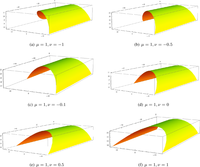

  

  Cubic enveloping developable GBT-Bézier surfaces for fixed μ

• 2. For fixed values of ν, the location of $J(0;\mu, \nu )$ and $J(1;\mu, \nu )$ will not fluctuate with fluctuating values of μ, but the lengths of ending generators $J(1;\mu, \nu )$ will modify. That is, the length of generators $J(1;\mu, \nu )$ increases with increasing value of μ and will be maximum at $\mu =1$, see Fig. 7.

  Figure 7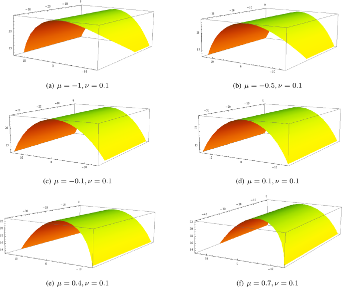

  

  Cubic enveloping developable GBT-Bézier surfaces designed for fixed ν

• 3. For identical values of $\mu, \nu$, the length and location of both starting $J(0;\mu, \nu )$ and ending $J(1;\mu, \nu )$ generators will modify with modifying values of $\mu, \nu$. With increasing values of $\mu, \nu$, the length of both generators increases. At the same instant, the structure of the enveloping developable surface will also modify as the height enveloping developable GBT-Bézier surface increases with decreasing values of $\mu, \nu$, see Fig. 8.

  Figure 8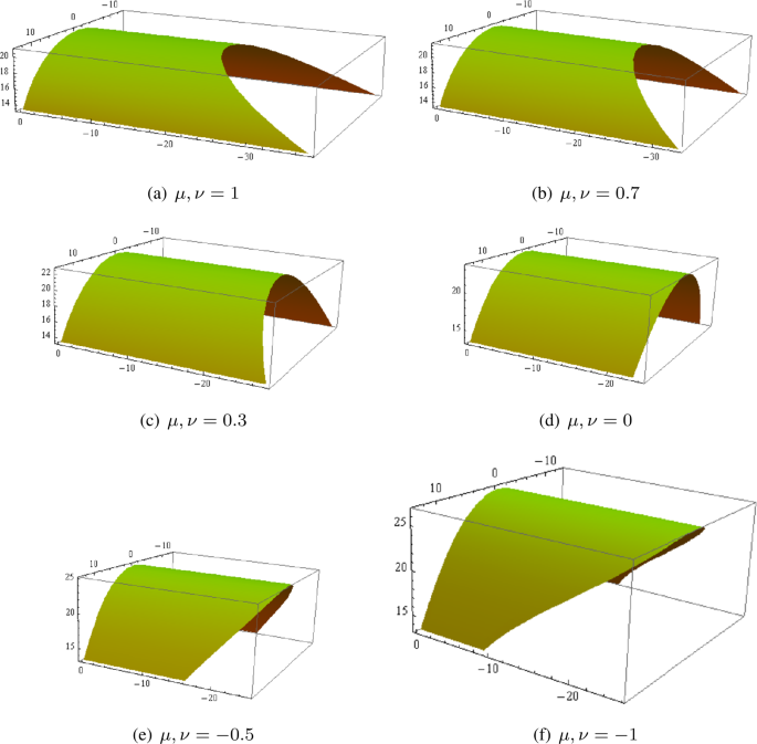

  

  Cubic enveloping developable GBT-Bézier surfaces for identical shape parameters

Example 4.2

In another construction of a developable GBT-Bézier surface, the control planes of the cubic enveloping developable GBT-Bézier surfaces are taken as follows:

$$\begin{aligned} \textstyle\begin{cases} {Q_{0}=(5\sqrt{2}, -5\sqrt{2}, 5, 125)}, \\ {Q_{1}=(-5\sqrt{2}, -5\sqrt{2}, 5, 125)}, \\ {Q_{2}=(-5\sqrt{2}, -5\sqrt{2}, 5, 125)}, \\ {Q_{3}=(5\sqrt{2}, -5\sqrt{2}, 5, 125)}. \end{cases}\displaystyle \end{aligned}$$

We can analyze from Figs. 9–12 that, with fluctuating values of shape parameters $\mu, \nu$, a class of enveloping developable GBT-Bézier surfaces can be designed on the requirement of provided control planes. A detailed effect of $\mu, \nu$ on the shape of an enveloping developable GBT-Bézier surface is described as follows:

• 1. When we fix the value of ν, the length of generator $J(1;\mu, \nu )$ will modify, but the location of generator $J(1;\mu, \nu )$ and the length and location of generator $J(0;\mu, \nu )$ will not modify with fluctuating values of μ. In other words, the length of the ending generator will increase simultaneously with an increase in the value of μ, see Figs. 9–10.

  Figure 9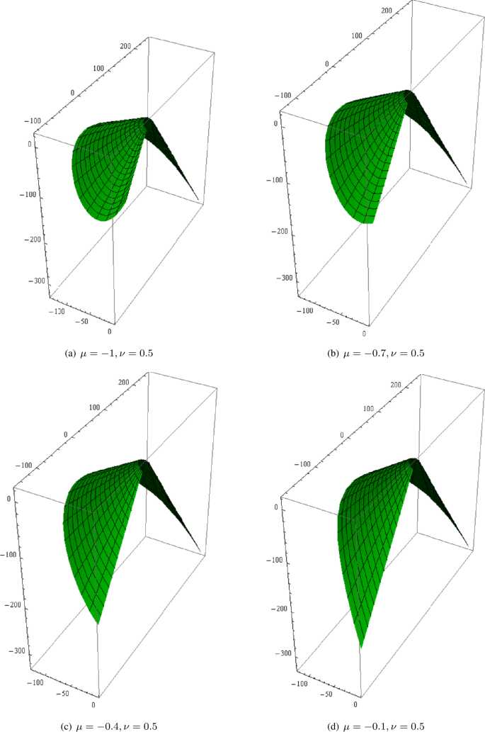

  

  The influence of parameters μ on cubic enveloping developable GBT-Bézier surface

  Figure 10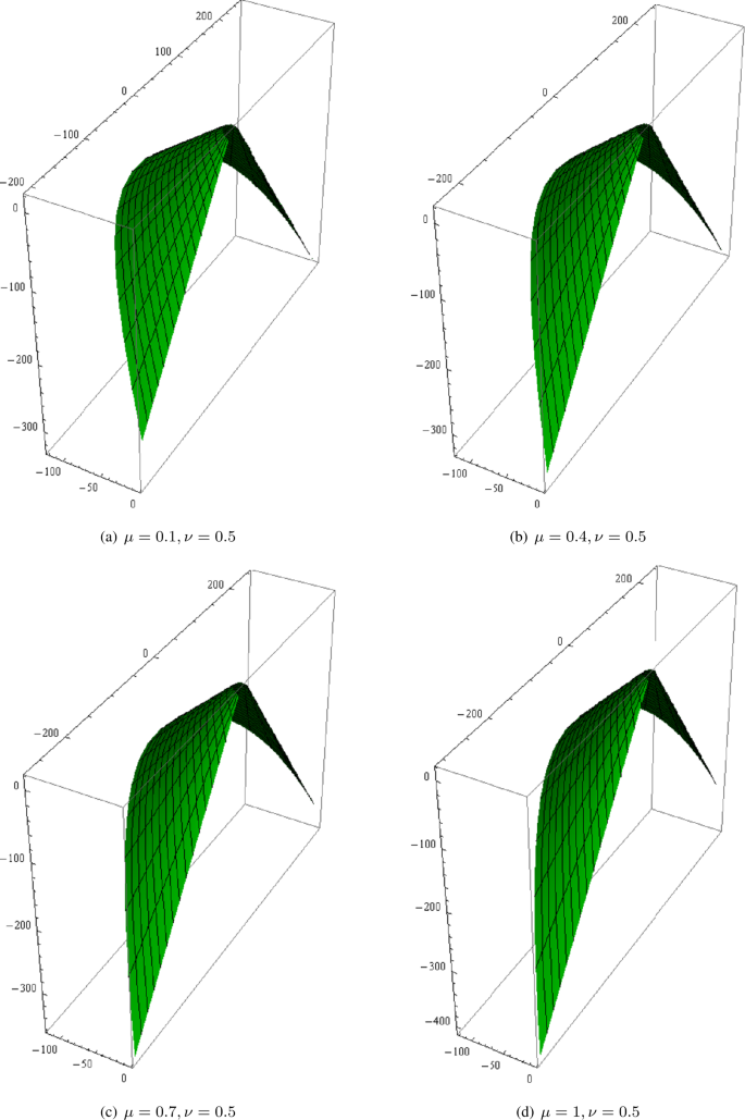

  

  The influence of parameters ν on cubic enveloping developable GBT-Bézier surface

• 2. When we take positive values of $\mu, \nu$, the length and location of $J(0;\mu, \nu )$ and location of $J(1;\mu, \nu )$ will not alter with the altering values of $\mu, \nu$, but the length of the ending generator $J(1;\mu, \nu )$ will modify, see Fig. 11.

  Figure 11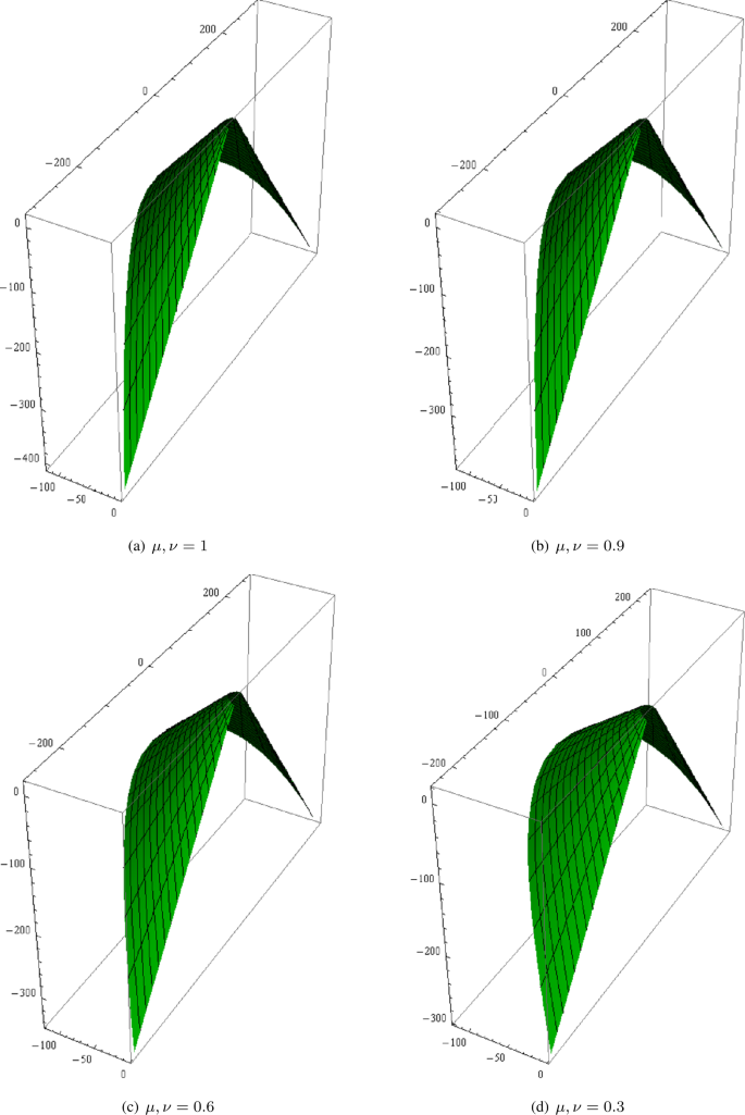

  

  The effects of positive values of shape parameters $\mu, \nu$ on cubic enveloping developable GBT-Bézier surface

• 3. When we take negative values of $\mu, \nu$, the location of $J(0;\mu, \nu )$ and $J(1;\mu, \nu )$ will not fluctuate with fluctuating values of $\mu, \nu$; however, the length of the ending and starting generator will modify along with the shape of the enveloping developable GBT-Bézier surface, see Fig. 12.

  Figure 12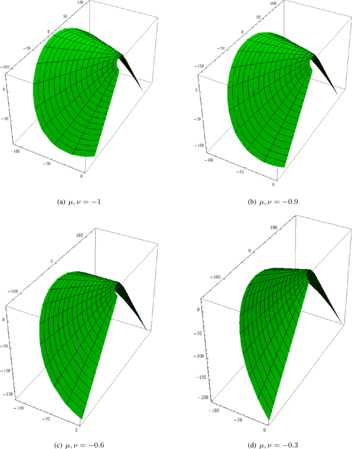

  

  The effects of negative values of shape parameters $\mu, \nu$ on cubic enveloping developable GBT-Bézier surface

4.2 Some designing examples of spine curve developable GBT-Bézier surfaces

To demonstrate the designing feature of a spine curve developable GBT-Bézier surface constructed from the tangent lines of the spine curve Sx, some design examples are given in this portion. For constructing a cubic spine curve developable GBT-Bézier surface, the central points of the control planes of a cubic spine curve developable GBT-Bézier surface are taken in four different quadrants I, II, III, IV with nonidentical distance from the origin, and the particular coordinates of control planes $Q_{0}$, $Q_{1}$, $Q_{2}$, $Q_{3}$ of a cubic spine curve developable GBT-Bézier surface are described as follows:

$$\begin{aligned} \textstyle\begin{cases} {Q_{0}=(6.5, 6.5, 6.5 \sqrt{2}, 169)}, \\ {Q_{1}=(-5.5, 7.5, 7.5 \sqrt{2}, 225)}, \\ {Q_{2}=(-10, -10, 10 \sqrt{2} 400)}, \\ {Q_{3}=(12.5, -12.5, 12.5 \sqrt{2}, 625)}. \end{cases}\displaystyle \end{aligned}$$

With different values of shape parameters μ and ν, a class of cubic spine curve developable GBT-Bézier surfaces can be designed on the requirement of provided control planes $Q_{0}$, $Q_{1}$, $Q_{2}$, $Q_{3}$ in Fig. 13 and Fig. 14 respectively, with distinct shapes.

Figure 13

Cubic spine curve developable GBT-Bézier surfaces designed by different values of ν

Figure 14

Cubic spine curve developable GBT-Bézier surfaces designed by different values of μ

5 Continuity requirements among developable GBT-Bézier surfaces

The designing of free-form complicated surfaces is a major issue in product designing, graphics, and CAD/CAM. In practical applications, the appearing design of many products is relatively complex and cannot be presented by an individual surface. Therefore, there is a requirement to construct these surfaces by using adjoining surfaces. The evaluation criteria for unwrinkled joining among two adjoining developable GBT-Bézier surfaces are $G^{1}$ and $G^{2}$ (Farin–Boehm and beta) continuity, etc. [15, 17, 21, 25, 30]. Now, we take an interpretation of GBT-Bézier curve having weight coefficients in 4D homogeneous space as

$$\begin{aligned} \hat{G}(x,\mu,\nu )=\sum^{k}_{i=0} g_{i,k}(x,\mu,\nu )\hat{R}_{i},\quad 0 \leq x\leq 1, \end{aligned}$$

(5.1)

where $g_{i,k}(z,\mu,\nu )\ (i=0,1,\ldots,k)$ are $k^{th}$ order GBTB basis functions; $\hat{R}=[\hat{R}_{0}, \hat{R}_{1},\ldots,\hat{R}_{k}]$, here $\hat{R}_{i}=(\omega _{i} R_{i}, \omega _{i})$ is the weighted control point of $R_{i}\ (i=0,1,\ldots,k)$ having weight factor $\omega _{i}$. It is understood that the weighted GBT-Bézier curve share the basic features with GBT-Bézier curves. When the weighted control points $\hat{R}_{i}=(\omega _{i} R_{i}, \omega _{i})\ (i=0,1,\ldots,k)$ in a 4D homogeneous space are considered as the control planes $Q_{i}\ (i=0,1,\ldots,k)$ in a 3D Euclidean space, the planes $\{\Pi _{x}\}$ constructed from control planes $Q_{i}\ (i=0,1,\ldots,k)$ are dual to the weighted GBT-Bézier curves constructed from $\hat{R}_{i}=(\omega _{i} R_{i}, \omega _{i})(i =0,1,\ldots,k)$. Hence some geometric design methods of developable GBT-Bézier surfaces (like continuity requirements, tangent planes, and terminal properties) in a 4D homogeneous space are identical to those of GBT-Bézier curves. Therefore, for continuity requirements of developable GBT-Bézier surfaces, it is imagined that the single parameter families of planes of two developable GBT-Bézier surfaces $H_{1}(x;\mu _{1},\nu _{1})$ and $H_{2}(x;\mu _{2},\nu _{2})$ of order k and l, respectively, that require to be joined together are defined as follows:

$$\begin{aligned} \textstyle\begin{cases} \{\Pi _{x,1}\}: H_{1}(x;\mu _{1},\nu _{1})={a_{0,1}(x), a_{1,1}(x), a_{2,1}(x), a_{3,1}(x)},\quad 0\leq x\leq 1, \\ \{\Pi _{x,2}\}: H_{2}(x;\mu _{2},\nu _{2})={a_{0,2}(x), a_{1,2}(x), a_{2,2}(x), a_{3,2}(x)}, \quad 0\leq x\leq 1, \end{cases}\displaystyle \end{aligned}$$

(5.2)

where $\mu _{i}, \nu _{i}\ (i=1, 2)$ are shape parameters and the control planes of $\{\Pi _{x,1}\}$ and $\{\Pi _{x,2}\}$ are $Q_{i,1}\ (i=0,1,\ldots,k)$ and $Q_{j,2}\ (j=0,1,\ldots,l)$, respectively.

5.1 $G^{1}$ continuity among developable GBT-Bézier surfaces

Here, we want to establish the first order geometric continuity or $G^{1}$ continuity among two or more weighted GBT-Bézier curves in a 4D homogeneous space. Now suppose that the single-parameter families of planes of the two contiguous weighted GBT-Bézier curves, which need to be spliced together, are as follows:

$$\begin{aligned} \textstyle\begin{cases} \hat{G}_{1}(x,\mu _{1},\nu _{1})=\sum^{k}_{i=0} g_{i,k}(x,\mu _{1}, \nu _{1})\hat{R}_{i,1},\quad 0\leq x\leq 1, \\ \hat{G}_{2}(x,\mu _{2},\nu _{2})=\sum^{l}_{j=0} g_{j,l}(x,\mu _{2}, \nu _{2})\hat{R}_{j,2}, \quad 0\leq x\leq 1, \end{cases}\displaystyle \end{aligned}$$

(5.3)

where $\mu _{i}, \nu _{i}\ (i=1,2)$ are shape parameters of two weighted GBT-Bézier curves $\hat{G}_{i}(x,\mu _{i}, \nu _{i})$ $(i=1, 2)$. $\hat{R}_{i,1}=(\omega _{i,1} R_{i,1}, \omega _{i,1})\ (i=0,1,\ldots,k)$ and $\hat{R}_{j,2}=(\omega _{j,2} Q_{j,2}, \omega _{j,2})\ (j=0,1,\ldots,l)$ are control points of $\hat{G}_{i}(x,\mu _{i}, \nu _{i})\ (i=1, 2)$, and $\omega _{i,1}\ (i=0,1,\ldots,k)$ and $\omega _{j,2}\ (j=0,1,\ldots,l)$ are weight factors of $\hat{G}_{i}(x,\mu _{i}, \nu _{i})\ (i=1, 2)$ respectively. Thus, from the definition of $G^{1}$ continuity among two parametric curves, the adequate and essential requirements for $G^{1}$ continuous connection among two or more contiguous weighted GBT-Bézier curves $\hat{G}_{1}(x)$ and $\hat{G}_{2}(x)$ are

$$\begin{aligned} \textstyle\begin{cases} \hat{G}_{2}(0,\mu _{2},\nu _{2})=\hat{G}_{1}(1,\mu _{1},\nu _{1}), \\ \hat{G}'_{2}(0,\mu _{2},\nu _{2})=\gamma \hat{G}'_{1}(1,\mu _{1},\nu _{1}), \end{cases}\displaystyle \end{aligned}$$

(5.4)

where $\gamma > 0$ is a constant. For control points $R_{i,j}\ (i=0,1,\ldots,k; j=1, 2)$ of two weighted GBT-Bézier curves $\hat{G}_{i}(x,\mu _{i}, \nu _{i})\ (i=1, 2)$ in a 4D homogeneous space understood as the control planes in 3D Euclidean space, the geometric continuity among two curves in a 4D homogeneous space certifies the geometric continuity among two conforming developable surfaces developed by using the duality principle in a 3D Euclidean space. Hence, from expression (5.4), the subsequent result can be acquired.

Theorem 2

Adequate and essential requirements for $G^{1}$ smooth connection among two contiguous developable GBT-Bézier surfaces $H_{1}(x,\mu _{1},\nu _{1})$ of order k and $H_{2}(x,\mu _{2},\nu _{2})$ of order l at the connection are

$$\begin{aligned} \textstyle\begin{cases} {Q_{0,2}=Q_{k,1}}, \\ {Q_{1,2}=Q_{k,1}+\gamma \frac{k-2+\frac{\pi }{2}(1+\nu _{1})}{l-2+\frac{\pi }{2}(1+\mu _{2})}(Q_{k,1}-Q_{k-1,1}).} \end{cases}\displaystyle \end{aligned}$$

(5.5)

Proof

If $H_{1}(x,\mu _{1},\nu _{1})$ and $H_{2}(x,\mu _{2},\nu _{2})$ want to reach $G^{1}$ continuity, it is compulsory that $H_{1}(x,\mu _{1},\nu _{1})$ and $H_{2}(x,\mu _{2},\nu _{2})$ reach $G^{0}$ continuity at the common first, which implies

$$\begin{aligned} Q_{0,2}=Q_{k,1}. \end{aligned}$$

(5.6)

In addition, $H_{1}(x,\mu _{1},\nu _{1})$ and $H_{2}(x,\mu _{2},\nu _{2})$ want to share a common tangent plane at connection, that is to say,

$$\begin{aligned} H'_{2}(0,\mu _{2},\nu _{2})=\gamma H'_{1}(1,\mu _{1},\nu _{1}). \end{aligned}$$

(5.7)

According to (3.11) and (3.12), we have

$$\begin{aligned} \textstyle\begin{cases} {H'_{1}(1,\mu _{1},\nu _{1})=(k-2+\frac{\pi }{2}(1+\nu _{1}))(Q_{k,1}-Q_{k-1,1}),} \\ {H'_{2}(0,\mu _{2},\nu _{2})=(l-2+\frac{\pi }{2}(1+\mu _{2}))(Q_{1,2}-Q_{0,2}).} \end{cases}\displaystyle \end{aligned}$$

(5.8)

Using (5.8) into (5.7), we get

$$\begin{aligned} \gamma \biggl(k-2+\frac{\pi }{2}(1+\nu _{1})\biggr) (Q_{k,1}-Q_{k-1,1})=\biggl(l-2+ \frac{\pi }{2} (1+\mu _{2})\biggr) (Q_{1,2}-Q_{0,2}). \end{aligned}$$

(5.9)

Ultimately, on the ground of (5.6), we can achieve

$$\begin{aligned} Q_{1,2}=Q_{k,1}+\gamma \frac{k-2+\frac{\pi }{2}(1+\nu _{1})}{l-2+\frac{\pi }{2}(1+\mu _{2})}(Q_{k,1}-Q_{k-1,1}). \end{aligned}$$

(5.10)

Hence equations (5.6) and (5.10) comprise the adequate and essential requirements of $G^{1}$ smooth connection betwixt two developable GBT-Bézier surfaces of order k and l sequentially. □

5.2 Farin–Boehm $G^{2}$ continuity requirements among developable GBT-Bézier surfaces

Now, we will derive the Farin–Boehm $G^{2}$ continuity requirements at the joints for the construction of piecewise developable GBT-Bézier surfaces. Similar to the $G^{1}$ continuity, when the control points of the two GBT-Bézier curves $\hat{G}_{1}(x,\mu _{1},\nu _{1})$, $\hat{G}_{2}(x,\mu _{2},\nu _{2})$ in a 4D homogeneous space are taken as control planes $Q_{i,j}\ (i=1,2,\ldots,k; j=1,2)$ in a 3D Euclidean space, then the Farin–Boehm $G^{2}$ continuity among two GBT-Bézier curves in a 4D homogeneous space ensures the Farin–Boehm $G^{2}$ continuity among two developable GBT-Bézier surfaces determined by $Q_{i,j}\ (i=1,2,\ldots,k; j=1,2)$ in a 3D Euclidean space [22]. Therefore, when two contagious developable GBT-Bézier surfaces in (5.2) want to reach Farin–Boehm $G^{2}$ continuity, they must satisfy the following requirements:

$$\begin{aligned} \textstyle\begin{cases} H_{2}(0,\mu _{2},\nu _{2})=H_{1}(1,\mu _{1},\nu _{1}), \\ H'_{2}(0,\mu _{2},\nu _{2})=H'_{1}(1,\mu _{1},\nu _{1}), \\ H''_{2}(0,\mu _{2},\nu _{2})=H''_{1}(1,\mu _{1},\nu _{1}). \end{cases}\displaystyle \end{aligned}$$

(5.11)

Equation (5.2) represents that the developable GBT-Bézier surfaces defined by $H_{1}(x, \mu _{1},\nu _{1})$, $H_{2}(x,\mu _{2},\nu _{2})$ need to have the same tangent plane, characteristic point, and generator at the joint.

Theorem 3

The essential and satisfactory requirements for achieving Farin–Boehm $G^{2}$ continuity betwixt two contiguous developable GBT-Bézier surfaces $H_{1}(x,\mu _{1},\nu _{1})$ of order k and $H_{2}(x,\mu _{2},\nu _{2})$ of order l at the connection are

$$\begin{aligned} \textstyle\begin{cases} Q_{0,2}=Q_{k,1}, \\ Q_{1,2}= Q_{k,1}+c(Q_{k,1}-Q_{k-1,1}), \\ Q_{2,2}=Q_{k,1}+c(Q_{k,1}-Q_{k-1,1})\\ \phantom{Q_{2,2}=}{} + \frac{1}{c_{l}+\pi ^{2}(1-\nu _{2})}[c_{k}(Q_{k,1}-2Q_{k-1,1}+Q_{k-2,1})- \pi ^{2}(1-\mu _{1}) \\ \phantom{Q_{2,2}=} {}\times (Q_{k-1,1}-Q_{k-2,1})+(2\pi ^{2}\nu _{1}+c(c_{l}+2 \pi ^{2}\mu _{2}))(Q_{k,1}-Q_{k-1,1})], \end{cases}\displaystyle \end{aligned}$$

(5.12)

where ${c= \frac{2(k-2)+\pi (1+\nu _{1})}{2(l-2)+\pi (1+\mu _{2})},}$ ${c_{k}=4(k-2)(k-3+\pi (1+\nu _{1}))}$, ${c_{l}=4(l-2)(l-3+\pi (1+\mu _{2})).}$

Proof

If $H_{1}(x,\mu _{1},\nu _{1})$ and $H_{2}(x,\mu _{2},\nu _{2})$ want to reach Farin–Boehm $G^{2}$ continuity, it is essential that $H_{1}(x,\mu _{1},\nu _{1})$ and $H_{2}(x,\mu _{2},\nu _{2})$ fulfil $G^{1}$ continuity at the joint boundary first, which implies

$$\begin{aligned} \textstyle\begin{cases} {Q_{0,2}=Q_{k,1}}, \\ {Q_{1,2}=Q_{k,1}+ \frac{2(k-2)+\pi (1+\nu _{1})}{2(l-2)+\pi (1+\mu _{2})}(Q_{k,1}-Q_{k-1,1}),} \end{cases}\displaystyle \end{aligned}$$

(5.13)

also

$$\begin{aligned} {H''_{2}(0,\mu _{2},\nu _{2})=H''_{1}(1, \mu _{1},\nu _{1}).} \end{aligned}$$

(5.14)

According to (3.11) and (3.12), we have

$$\begin{aligned} &4(l-2) \bigl(l-3+\pi (1+\mu _{2})\bigr) (Q_{0,2}-2Q_{1,2}+Q_{2,2})+2\pi ^{2}\mu _{2}(Q_{0,2}-Q_{1,2}) \\ &\quad{}- \pi ^{2}(1-\nu _{2}) (Q_{1,2}-Q_{2,2})=4(k-2) \\ &\quad{}\times \bigl(k-3+\pi (1+\nu _{1})\bigr) (Q_{k-2,1}-2Q_{k-1,1}+Q_{k,1}) \\ &\quad{}+ \pi ^{2}(1-\mu _{1}) (Q_{k-2,1}-Q_{k-1,1}) -2 \pi ^{2}\nu _{1}(Q_{k-1,1}-Q_{k,1}). \end{aligned}$$

(5.15)

Simply by using the values of $Q_{0,2},Q_{1,2}$ from expression (5.6) into expression (5.8), we can get the required Farin–Boehm $G^{2}$ continuity requirements (5.5). □

5.3 $G^{2}$ beta continuity among developable GBT-Bézier surfaces

Theorem 4

For a smooth continuous connection among two adjoining developable GBT-Bézier surfaces $H_{1}(x,\mu _{1},\nu _{1})$ and $H_{2}(x,\mu _{2},\nu _{2})$ of order k and l, respectively, the necessary and sufficient $G^{2}$ beta continuity requirements are

$$\begin{aligned} \textstyle\begin{cases} Q_{0,2}=Q_{k,1}, \\ Q_{1,2}=Q_{k,1}+c\gamma (Q_{k,1}-Q_{k-1,1}), \\ Q_{2,2}=Q_{k,1}+c\gamma (Q_{k,1}-Q_{k-1,1})\\ \phantom{Q_{2,2}=}{} + \frac{1}{c_{l}+\pi ^{2}(1-\nu _{2})}[c_{k}\gamma ^{2}(Q_{k,1}-2Q_{k-1,1}+Q_{k-2,1})- \pi ^{2}\gamma ^{2}(1-\mu _{1}) \\ \phantom{Q_{2,2}=}{}\times (Q_{k-1,1}-Q_{k-2,1})+(\gamma (2\pi ^{2} \nu _{1}\gamma +\mathit{cc}_{l}+2c\pi ^{2}\mu _{2})\\ \phantom{Q_{2,2}=}{}+\lambda (k-2+\frac{\pi }{2}(1+ \nu _{1}))) (Q_{k,1}-Q_{k-1,1})], \end{cases}\displaystyle \end{aligned}$$

(5.16)

where ${c= \frac{2(k-2)+\pi (1+\nu _{1})}{2(l-2)+\pi (1+\mu _{2})},}$ ${c_{k}=4(k-2)(k-3+\pi (1+\nu _{1}))}$, ${c_{l}=4(l-2)(l-3+\pi (1+\mu _{2})).}$

Proof

To reach $G^{2}$ beta continuity among $H_{1}(x,\mu _{1},\nu _{1})$ and $H_{2}(x,\mu _{2},\nu _{2})$, there are some subsequent requirements which must be satisfied at the common boundary

$$\begin{aligned} \textstyle\begin{cases} {Q_{0,2}= H_{2}(0,\mu _{2},\nu _{2})=H_{1}(1,\mu _{1}, \nu _{1})=Q_{k,1},} \\ H'_{2}(0,\mu _{2},\nu _{2})=\gamma H'_{1}(1,\mu _{1}, \nu _{1}), \quad \gamma >0, \\ {H''_{2}(0,\mu _{2},\nu _{2})= \gamma ^{2} H''_{1}(1, \mu _{1},\nu _{1})+\lambda H'_{1}(1,\mu _{1},\nu _{1}),} \end{cases}\displaystyle \end{aligned}$$

(5.17)

where $\gamma >0$ and λ are constants. From the terminal properties of developable GBT-Bézier surfaces and substituting expressions (3.11) and (3.12) into expression (5.17), we can achieve $G^{2}$ beta continuity expression (5.16). Hence the three equations of expression (5.16) establish the adequate and essential requirements of $G^{2}$ beta continuity requirements among two or more developable GBT-Bézier surfaces. □

5.4 Steps for smooth continuous connection between two adjacent developable GBT-Bézier surfaces

Using smooth continuity requirements among two contiguous developable surfaces, a huge amount of complicated surfaces can be made easily. To show $G^{2}$ smooth continuity (Farin–Boehm and beta) steps betwixt two adjoining developable GBT-Bézier surfaces, an example is used here. For establishing a $G^{2}$ beta continuous connection among two or more contiguous cubic enveloping developable GBT-Bézier surfaces, the following steps are performed.

Step 1. Preliminary developable GBT-Bézier surface $H_{1}(x; \mu _{1}, \nu _{1})$, its control planes $Q_{i,1}\ (i=0,1,2,3)$, and shape parameters $\mu _{1}, \nu _{1}$ can be given openly.

Step 2. Let $Q_{k,1}=Q_{0,2}$, or in other words, the developable GBT-Bézier surfaces expressed by $H_{1}(x; \mu _{1}, \nu _{1})$ and $H_{2}(x; \mu _{2}, \nu _{2})$) have a combined control plane to fulfil the $G^{0}$ continuity condition.

Step 3. For any provided values of $\mu _{2}, \nu _{2}$ and constant $\gamma >0$, the 2nd control plane $Q_{1,2}$ of the developable GBT-Bézier surface $H_{2}(x; \mu _{2}, \nu _{2})$ can be calculated from the second equation of (5.16).

Step 4. From the $3rd$ equation of (5.16), the control plane $Q_{2,2}$ of the developable GBT-Bézier surface $H_{2}(x; \mu _{2},\nu _{2})$ can be determined on the bases of Step 2 and Step 3 for a defined value of constant λ.

Step 5. The last control plane $Q_{3,2}$ of $H_{2}(x; \mu _{2}, \nu _{2})$ can be selected openly for establishing $G^{2}$ beta smooth continuous connection among two or more adjoining developable GBT-Bézier surfaces.

From iteration of the above steps among two developable GBT-Bézier surfaces, $G^{2}$ beta smooth continuity can be attained among multiple developable GBT-Bézier surfaces, and it can also be applied on other continuity conditions in the same manners.

5.5 Some modeling examples of smooth developable GBT-Bézier surfaces

This portion will give some designing examples of $G^{2}$ smooth connection (beta and Farin–Boehm) among two adjoining cubic developable GBT-Bézier surfaces sequentially. Additionally, the effect of shape parameters on combined surfaces is also examined.

Example 5.1

Figures 15–16 exhibit the graphs of Farin–Boehm $G^{2}$ continuity among two adjoining cubic enveloping developable GBT-Bézier surfaces. In these figures, the blue surfaces are primary developable GBT-Bézier surfaces with subsequent control planes

$$\begin{aligned} \textstyle\begin{cases} {Q_{0,1}=(0, -20, 10, 400)}, \\ {Q_{1,1}=(0, -10, 20, 400)}, \\ {Q_{2,1}=(0, 10, 20, 400)}, \\ {Q_{3,1}=(0, 20, 10, 400)}. \end{cases}\displaystyle \end{aligned}$$

(5.18)

The green surfaces are the secondary enveloping developable GBT-Bézier surfaces. For all spliced surfaces, the last control plane $Q_{3,2}$ is given openly, and the first three control planes are derived from Farin–Boehm $G^{2}$ continuity conditions. Figure 15 demonstrates the influence of shape parameter μ on combined developable GBT-Bézier surfaces with fixed value of ν. These four graphs indicate that without disturbing control planes, the shape of the combined developable GBT-Bézier surface can be simply modified by amending the shape parameters. Figure 16 represents the impact of shape parameter ν on the combined developable GBT-Bézier surface for a fixed value of μ.

Figure 15

Farin–Boehm $G^{2}$ continuity among two cubic enveloping developable GBT-Bézier surfaces

Figure 16

Farin–Boehm $G^{2}$ continuity betwixt two cubic enveloping developable GBT-Bézier surfaces

Example 5.2

Geometric design of $G^{2}$ beta continuity among two contiguous cubic enveloping developable GBT-Bézier surfaces is illustrated in Fig. 17. In Fig. 17, the green surface represents first cubic enveloping developable GBT-Bézier surface $H1(x;\mu _{1}, \nu _{1})$ with control planes described in (5.18), whereas red surface represents the 2nd cubic enveloping developable GBT-Bézier surface $H2(x;\mu _{2}, \nu _{2})$ which fulfills the $G^{2}$ beta continuity requirements with $H1(x;\mu 1, \nu 1)$. By setting all shape parameters $\mu _{1}, \nu _{1}, \mu _{2}, \nu _{2}$ of the corresponding cubic enveloping developable GBT-Bézier surfaces equal to 1, the coordinates of the control planes of cubic enveloping developable GBT-Bézier surface $H2(x;\mu _{2}, \nu _{2})$ are calculated as follows:

$$\begin{aligned} \textstyle\begin{cases} {Q_{0,2}=(0, 20, 10, 400)}, \\ {Q_{1,2}=(0, 30, 0, 400)}, \\ {Q_{2,2}=(0, 45.708, -35.708, 400)}, \end{cases}\displaystyle \end{aligned}$$

where the last control plane $Q_{3,2}$ is given without restraint, and the control planes $Q_{0,2}, Q_{1,2}, Q_{2,2}$ are calculated according to (5.16) ($\gamma =1, \lambda =0$). Figure 17 represents the combined enveloping developable GBT-Bézier surface having $G^{2}$ beta connection among them after amending the values of its shape parameters, while Fig. 18 indicates the combined enveloping developable GBT-Bézier surface for multiple values of scale factor γ. Figure 18 indicates that a unified merged developable GBT-Bézier surface can be achieved by setting scaling factor $\gamma =1$, unconcerned of modifying the shape parameter, and at connection a gap will be achieved on merged developable GBT-Bézier surfaces when $\gamma \neq 1$. We can use these characteristics to design a complex surface according to our needs.

Figure 17

$G^{2}$ beta smooth continuity among two cubic developable GBT-Bézier surfaces

Figure 18

The effects of scale factor λ on composite developable GBT-Bézier surface with $G^{2}$ beta smooth continuity

6 Conclusions

In this research work, developable GBT-Bézier surfaces (enveloping developable and spine curve developable) along two shape parameters have been proposed. The geometric features and influence role of shape parameters on these newly constructed developable GBT-Bézier surfaces have been examined. Additionally, the geometric continuity requirements ($G^{1}$, $G^{2}$ Farin–Boehm and $G^{2}$ beta) among two contiguous developable GBT-Bézier surfaces have been derived for the construction of complicated developable GBT-Bézier surfaces. These proposed developable GBT-Bézier surfaces have been shown to reduce the flaws of line and plane geometric description in modeling developable GBT-Bézier surface design, and we proved that they are more beneficial than the actual developable Bézier surfaces. In contrast with other Bézier curves and surfaces techniques having multiple shape parameters, our interpretation of basis functions determined in this research is simple and extra succinct.

References

Chung, W., Kim, S.H., Shin, K.H.: A method for planar development of 3D surfaces in shoe pattern design. J. Mech. Sci. Technol. 22, 1510–1519 (2008)
Liu, Y., Pottman, H., Wallner, J., et al.: Geometric modeling with conical meshes and developable surfaces. ACM Trans. Graph. 25(3), 681–689 (2006)
Tang, C., Bo, P., Wallner, J., Pottman, H.: Interactive design of developable surfaces. ACM Trans. Graph. 35(2), 1–12 (2016)
Aumann, G.: Interpolation with developable Bézier patches. Comput. Aided Geom. Des. 8(5), 409–420 (1991)
Aumann, G.: A simple algorithm for designing developable Bézier surfaces. Comput. Aided Geom. Des. 20(8), 601–619 (2003)
Aumann, G.: Degree elevation and developable Bézier surfaces. Comput. Aided Geom. Des. 21(7), 661–670 (2004)
Zhang, X.W., Wang, G.J.: A new algorithm for designing developable Bézier surfaces. J. Zhejiang Univ. Sci. 7(12), 2050–2056 (2006)
Fernandez, J.: B-spline control nets for developable surfaces. Comput. Aided Geom. Des. 24(4), 189–199 (2007)
Chu, C.H., Wang, C., Tsai, C.R.: Computer aided geometric design of strip using developable Bézier patches. Comput. Ind. 59(6), 601–611 (2008)
Hwang, H.D., Yoon, S.H.: Constructing developable surfaces by wrapping cones and cylinders. Comput. Aided Des. 58, 230–235 (2015)
Bodduluri, R., Ravani, B.: Design of developable surfaces using duality between plane and point geometries. Comput. Aided Des. 25(10), 621–632 (1993)
Bodduluri, R., Ravani, B.: Geometric design and fabrication of developable Bézier and B-spline surfaces. J. Mech. Des. 116(4), 1042–1048 (1994)
Pottmann, H., Farin, G.: Developable rational Bézier and B-spline surfaces. Comput. Aided Geom. Des. 12(5), 513–531 (1995)
Pottmann, H., Wallner, J.: Approximation algorithms for developable surfaces. Comput. Aided Geom. Des. 16(6), 539–556 (1999)
Zhou, M., Peng, G.H., Ye, Z.L.: Design of developable surfaces by using duality between plane and point geometries. J. Comput.-Aided Des. Comput. Graph. 16(10), 1401–1406 (2004)
Zhou, M., Peng, G., Ye, Z., An, X., Wang, S.: Geometric design of adjustably developable surfaces. Chin. J. Mech. Eng. 18(12), 1425–1429 (2007)
Zhou, M., Yang, J.Q., Zheng, H.C., Song, W.J.: Design and shape adjustment of developable surfaces. Appl. Math. Model. 37, 3789–3801 (2013)
Li, C.Y., Zhu, C.G.: \(G^{1}\) continuity of four pieces of developable surfaces with Bézier boundaries. Comput. Appl. Math. 329, 164–172 (2017)
Chu, C.H., Chen, J.T.: Geometric design of developable composite Bézier surfaces. Comput-Aided Des. Appl. 1(1–4), 531–539 (2004)
Jüttler, B., Sampoli, M.L.: Hermite interpolation by piecewise polynomial surfaces with rational offsets. Comput. Aided Geom. Des. 17(4), 361–385 (2000)
Hu, G., Cao, H., Qin, X., Wang, X.: Geometric design and continuity conditions of developable λ-Bézier surfaces. Adv. Eng. Softw. 114, 235–245 (2017)
Hu, G., Cao, H., Zhang, S., Wei, G.: Developable Bézier-like surfaces with multiple shape parameters and its continuity conditions. Appl. Math. Model. 45, 728–747 (2017)
Hu, G., Junli, W., Qin, X.Q.: A new approach in designing of local controlled developable H-Bézier surfaces. Adv. Eng. Softw. 121, 26–38 (2018)
Hu, G., Junli, W.: Generalized quartic H-Bézier curves: construction and application to developable surfaces. Adv. Eng. Softw. 138, 1–15 (2019)
Hu, G., Cao, H., Wu, J., Wei, G.: Construction of developable surfaces using generalized C-Bézier bases with shape parameters. Comput. Appl. Math. 39, 1–32 (2020)
Kusno: Construction of regular developable Bézier patches. Math. Comput. Appl. 24, 1–13 (2019)
Li, C., Zhu, C.: Designing developable C-Bézier surface with shape parameters. Mathematics 8(3), 1–21 (2020)
Hu, G., Li, H., Hu, X.: A novel geometric modeling approach for cubic developable C-Bézier surfaces. J. Adv. Mech. Des. Syst. Manuf. 14, 1–14 (2020)
Ammad, M., Misro, M.Y., Abbas, M., Majeed, A.: Generalized developable cubic trigonometric Bézier surfaces. Mathematics 9(3), 283 (2021)
Farin, G.: Curves and Surfaces for CAGD: A Practical Guide. 5th edn. Acadezmic Press, San Diego (2002)
Sidra, M., Abbas, M., Miura, K.T., Majeed, A., Iqbal, A.: Geometric modeling and applications of generalized blended trigonometric Bernstein-like polynomial functions. Adv. Differ. Equ. 2020, 550 (2020)
Acknowledgements
We thank Dr. Muhammad Amin for his assistance in proofreading of the manuscript. This research was supported by the Department of Mechanical Engineering, Shizuoka University, Hamamatsu, 432-8561 Shizuoka, Japan.
Funding
No external funding is available for this research.
Author information
Authors and Affiliations
Contributions
All authors equally contributed to this work. All authors read and approved the final manuscript.
Corresponding author
Ethics declarations
Competing interests
The authors declare that they have no competing interests.
Rights and permissions
Open Access This article is licensed under a Creative Commons Attribution 4.0 International License, which permits use, sharing, adaptation, distribution and reproduction in any medium or format, as long as you give appropriate credit to the original author(s) and the source, provide a link to the Creative Commons licence, and indicate if changes were made. The images or other third party material in this article are included in the article’s Creative Commons licence, unless indicated otherwise in a credit line to the material. If material is not included in the article’s Creative Commons licence and your intended use is not permitted by statutory regulation or exceeds the permitted use, you will need to obtain permission directly from the copyright holder. To view a copy of this licence, visit http://creativecommons.org/licenses/by/4.0/.
About this article
Cite this article
Maqsood, S., Abbas, M., Miura, K.T. et al. Shape-adjustable developable generalized blended trigonometric Bézier surfaces and their applications. Adv Differ Equ 2021, 459 (2021). https://doi.org/10.1186/s13662-021-03614-3
Received:
Accepted:
Published:
DOI: https://doi.org/10.1186/s13662-021-03614-3