On a geometric study of a class of normalized functions defined by Bernoulli’s formula

Abstract

The central purpose of this effort is to investigate analytic and geometric properties of a class of normalized analytic functions in the open unit disk involving Bernoulli’s formula. As a consequence, some solutions are indicated by the well-known hypergeometric function. The class of starlike functions is investigated containing the suggested class.

1 Introduction

Ma and Minda offered a couple classes of starlike and convex normalized functions in the open unit disk. They defined these classes utilizing the theory of differential subordination. Later, the Ma–Minda classes were considered by many investigators. Furthermore, the researchers established different classes containing different types of linear, differential, and integral operators [1]. Denote the class of analytic functions in the open unit disk by $\mathcal{H}(\cup )$, and for $\hbar \in \mathbb{C}$, we define the class

$$ \mathcal{H}[\varsigma ,k]= \bigl\{ \psi \in \mathcal{H}(\cup ): \psi (\xi )= \varsigma +\varsigma _{k}\xi ^{k}+\varsigma _{k+1}\xi ^{k+1}+\cdots\bigr\} . $$

Define a subclass of $\mathcal{H}[0,1]$ as follows:

$$ \wedge := \bigl\{ \sigma \in \mathcal{H}[0,1]: \sigma (0)=0, \sigma ' (0)=1 \bigr\} . $$

For a normalized analytic function $\sigma (\xi ) \in \wedge$, $\xi \in \cup :=\{\xi \in \mathbb{C}: | \xi |<1 \}$ satisfying the power series

$$ \sigma (\xi )= \xi +\sum_{n=2}^{\infty } a_{n} \xi ^{n}, \quad \xi \in \cup , $$

(1.1)

the Ma–Minda starlike class $(\mathcal{M}^{*})$ is defined as follows:

$$ \frac{\xi \sigma ' (\xi )}{\sigma (\xi )} \prec \varsigma (\xi ), \quad \xi \in \Xi \Leftrightarrow \Re \biggl( \frac{\xi \sigma ' (\xi )}{\sigma (\xi )} \biggr)> \wp , \wp \in [0,1), $$

(1.2)

where ς is an analytic function with positive real part on Ξ, $\varsigma (0) = 1$, $\varsigma ^{\prime }(0) > 0$, and ς maps Ξ onto a starlike domain corresponding to ∂Ξ and symmetric with respect to the real axis. The symbol ≺ is presented as the notion of the subordination (see [2]). Moreover, the Ma–Minda convex class $(\mathcal{M}^{c} )$ is formulated by the subordination inequality

$$ 1+ \frac{\xi \sigma '' (\xi )}{\sigma ' (\xi )} \prec \varsigma (\xi ), \quad \xi \in \cup \Leftrightarrow \Re \biggl(1+ \frac{\xi \sigma '' (\xi )}{\sigma '(\xi )} \biggr)> \wp , \wp \in [0,1). $$

(1.3)

A linear combination of these two classes is formulated by using different types of analytic functions including differential, integral, and linear operators and transformations (see for recent studies [3–12]).

In this note, we suggest to study the general formula of Bernoulli’s equation in a complex domain. We formulate an integral operator and a transform convoluted with a special function concerning Bernoulli’s formula subordinated with a class of analytic functions. We present sufficient conditions to be a starlike function. Special cases are illustrated in the sequel.

2 Bernoulli’s formula

In this section, we present a special type of Bernoulli’s equation as follows:

$$ \biggl(\frac{\xi }{\sigma (\xi )} \biggr)- \biggl( \frac{\xi }{\sigma (\xi )} \biggr)^{2} \sigma '(\xi )-2=0, \quad \xi \in \cup , \sigma \in \wedge . $$

(2.1)

The solution of (2.1) is given by

$$\begin{aligned} \sigma (\xi ) &=\frac{\xi }{c \xi ^{2} + 1} \\ &= \sum_{n=0}^{\infty } \frac{ ((1 + \sqrt{ \vert c \vert }) (\frac{\sqrt{ \vert c \vert } - c}{1 + c} )^{n} + (-1 + \sqrt{ \vert c \vert }) (-\frac{\sqrt{ \vert c \vert } - c}{1 + c} )^{n} ) ( \xi -1)^{n}}{2 (\sqrt{ \vert c \vert } (1 + c) )} \\ &=\xi - c \xi ^{3} + c^{2} \xi ^{5} + O \bigl(\xi ^{7}\bigr), \quad \vert \xi \vert < \frac{1}{\sqrt{ \vert c \vert }}, c\neq 0. \end{aligned}$$

A first generalization of (2.1) is formulated by considering a convex formula

$$ (1-\alpha ) \biggl(\frac{\xi }{\sigma (\xi )} \biggr)+\alpha \biggl( \frac{\xi }{\sigma (\xi )} \biggr)^{2} \sigma '(\xi )-1=0, \quad \xi \in \cup , \sigma \in \wedge , $$

(2.2)

where $\alpha \in [0,1]$ taking the solution formula

$$ \sigma (\xi ) =\frac{\xi }{c \xi ^{1/\alpha } + 1}. $$

It is clear that when $\alpha =0.5$, Eq. (2.2) reduces to Eq. (2.1). The most parametric Bernoulli’s equation is given by

$$ (1-\alpha ) \biggl(\frac{\xi }{\sigma (\xi )} \biggr)^{\beta }+ \alpha \biggl(\frac{\xi }{\sigma (\xi )} \biggr)^{\beta +1} \sigma '(\xi )-1=0, \quad \xi \in \cup , \sigma \in \wedge , $$

(2.3)

having the solution

$$ \sigma (\xi )= \frac{1}{ (-\xi ^{-\beta } (-e^{\beta c} \xi ^{\beta /\alpha } - 1) )^{1/\beta }}= \frac{1}{ (\xi ^{-\beta } (1 +\xi ^{\beta /\alpha } \sum_{n=0}^{\infty }\frac{ (\beta c)^{n}}{n!} ) )^{1/\beta }}=\xi+\cdots . $$

When $\beta \in [0, \alpha )$, Bernoulli’s formula is studied early [13, 14]. In this effort, we consider $\beta \in [1,\infty )$ and hence, for $\beta =2$, we have two solutions as follows:

$$ \sigma (\xi ) = \pm \frac{\xi }{\sqrt{c \xi ^{2/\alpha } + 1}}; $$

and for $\beta =3$, we get three different solutions

$$ \sigma _{1}(\xi ) =\frac{\xi }{(c \xi ^{3/\alpha } + 1)^{1/3}}, \qquad \sigma _{2}(\xi ) =- \frac{(-1)^{1/3}\xi }{(c \xi ^{3/\alpha } + 1)^{1/3}}, \qquad \sigma _{3}( \xi ) =\frac{(-1)^{2/3}\xi }{(c \xi ^{3/\alpha } + 1)^{1/3}}. $$

More generalization can be viewed by consider the following equation:

$$ (1-\alpha ) \biggl(\frac{\xi }{\sigma (\xi )} \biggr)^{\beta }+ \alpha \biggl(\frac{\xi }{\sigma (\xi )} \biggr)^{\beta +1} \sigma '(\xi )-1= \lambda (\xi ). $$

(2.4)

For example, let $\lambda (\xi )=\xi$ (starlike in ∪), then Eq. (2.4) admits a unique solution satisfying the equation

$$ c= \frac{\alpha ^{2} \xi ^{\frac{(\alpha - 1) \beta }{\alpha }} \sigma (\xi )^{-\beta } ( (\frac{\xi }{\alpha - \beta } - \frac{1}{\beta } ) (\frac{\xi }{\sigma (\xi )} )^{-\beta } +\frac{ 1}{\beta } )}{(1-\alpha ) \beta }, \quad \alpha \neq \beta . $$

Also, let $\lambda (\xi )=e^{\xi }-1$, which is starlike in ∪ (see [2], p.270), then the solution becomes

$$ c= \frac{\alpha ^{2} \xi ^{\frac{(\alpha - 1) \beta }{\alpha }} (\frac{\xi }{\sigma (\xi )} )^{-\beta } \sigma (\xi )^{-\beta } (\alpha (\frac{\xi }{\sigma (\xi )} )^{\beta }- \beta (-\xi )^{\beta /\alpha } \Gamma (-\frac{\beta }{\alpha },-\xi ) )}{(1-\alpha ) \beta ^{2}}, $$

where Γ indicates the incomplete gamma function. We proceed to suggest a class of analytic functions taking the Ma–Minda design as follows.

Definition 2.1

Let $\sigma \in \wedge$. For two parameters $\alpha \in [0,1]$ and $\beta \in [1,\infty )$ and a function $\lambda \in \wedge$ satisfying

$$ (1-\alpha ) \biggl(\frac{\xi }{\sigma (\xi )} \biggr)^{\beta }+ \alpha \biggl(\frac{\xi }{\sigma (\xi )} \biggr)^{\beta +1} \sigma '(\xi )-1 \prec \lambda (\xi ). $$

(2.5)

The set of all these functions is denoted by $\mathcal{M}^{\alpha ,\beta }(\lambda )$.

The aim of the above class is to dominate the normalized solution of Bernoulli’s equation by another normalized function in ∧.

3 Geometric results

This section deals with $\Re (\Theta (\xi ) ):= \Re ((1-\alpha ) ( \frac{\xi }{\sigma (\xi )} )^{\beta }+\alpha ( \frac{\xi }{\sigma (\xi )} )^{\beta +1} \sigma '(\xi )-1 )$.

Theorem 3.1

Consider the class $\mathcal{M}^{\alpha ,\beta }(\lambda )$. Define a functional

$$\begin{aligned} \Theta (\xi ) &= (1-\alpha ) \biggl(\frac{\xi }{\sigma (\xi )} \biggr)^{ \beta }+ \alpha \biggl(\frac{\xi }{\sigma (\xi )} \biggr)^{\beta +1} \sigma '(\xi )-1 \\ &=\xi +\sum_{n=2}^{\infty }\phi _{n} \xi ^{n}, \quad \xi \in \cup . \end{aligned}$$

If $\Re (\Theta (\xi ) )>0$, then

$$ \vert \phi _{n} \vert \leq 2 \int _{0}^{2\pi } \bigl\vert e^{-in\theta } \bigr\vert \,d\mu (\theta ), \quad n \geq 2, $$

where dμ is a probability measure. Moreover, if $\Re (e^{i \varpi }\Theta (\xi ) )>0$, then

$$ \lambda (\xi )= \frac{(A-B)\xi }{1+B\xi } \in \mathcal{C}, \quad \vert A \vert =1, \vert B \vert =1, $$

where $\mathcal{C}$ is the class of analytic convex in ∪.

Proof

For the first part of the theorem, we suppose that

$$ \Re \bigl(\Theta (\xi )+1\bigr)= \Re \Biggl(1+\sum_{n=1}^{\infty } \phi _{n} \xi ^{n} \Biggr)>0, \quad \phi _{1}=1. $$

Then, by the Carathéodory positivist method for analytic functions, we have

$$ \vert \phi _{n} \vert \leq 2 \int _{0}^{2\pi } \bigl\vert e^{-in\theta } \bigr\vert d\mu (\theta ), \quad n \geq 2, $$

where dμ is a probability measure. For the second part, we have the assumption

$$ \Re \bigl(e^{i \varpi }\bigl(1+\Theta (\xi )\bigr) \bigr)>0, \quad \xi \in \cup , \varpi \in \mathbb{R}. $$

Then, according to [15]-Theorem 1.6(P22) and for some real numbers ϖ, we obtain

$$ \bigl[\Theta (\xi )\bigr] +1 \approx \frac{A \xi +1}{B\xi +1}, \quad \xi \in \cup , $$

or $\lambda (\xi )= \frac{(A-B)\xi }{1+B\xi }$. But $\frac{A\xi +1}{B \xi +1}$ is convex in ∪, then we obtain that $\lambda (\xi ) \in \mathcal{C}$. □

The next theorem is the converse of Theorem 3.1.

Theorem 3.2

Consider the functional $[\Theta (\xi )]=(1-\alpha ) (\frac{\xi }{\sigma (\xi )} )^{ \beta }+\alpha (\frac{\xi }{\sigma (\xi )} )^{\beta +1} \sigma '(\xi )-1$, where $\sigma \in \wedge$. Then the subordination

$$\begin{aligned}& \frac{\beta [\Theta (\xi )] ([\Theta (\xi )] +1)+\xi [\Theta (\xi )]' }{\beta ([\Theta (\xi )] +1)} \prec \frac{A\xi +1}{B\xi +1} \\& \quad \bigl(\alpha \in [0,1], \beta \in [1,\infty ), B \in [-1,0], A \in (0,1], \xi \in \cup \bigr) \end{aligned}$$

implies $\sigma \in \mathcal{M}^{\alpha ,\beta }(\frac{(A-B)\xi }{1+B\xi })$. Moreover, the subordination

$$ \sigma (\xi )+\xi \sigma ' (\xi ) \bigl(\beta \sigma (\xi )+ \alpha \bigr)\prec \frac{(A-B)\xi }{1+B\xi } $$

yields $\sigma (\xi )\prec \lambda (\xi )=\frac{(A-B)\xi }{1+B\xi }$.

Proof

Let $p(\xi ):=[\Theta (\xi )] +1$. Then a computation gives

$$\begin{aligned} p(\xi )+ \frac{\xi p' (\xi )}{\beta (p(\xi )+1)}&= \bigl(\bigl[\Theta ( \xi )\bigr] +1 \bigr) \biggl( \frac{\xi [\Theta (\xi )]' }{\beta ( [\Theta (\xi )] +1 )} \biggr) \\ &= \frac{\beta [ \Theta (\xi )] ([\Theta (\xi )] +1 ) +\xi [ \Theta (\xi )] ' }{\beta ([\Theta (\xi )] +1 )} \\ &\prec \frac{A\xi +1}{B\xi +1}. \end{aligned}$$

According to [2]-Theorem 3.3d., we have

$$ \Theta (\xi )+1 \prec \frac{A\xi +1}{B\xi +1}. $$

That is, $\sigma \in \mathcal{M}^{\alpha ,\beta }(\frac{(A-B)\xi }{1+B\xi })$.

Now, since $\Re ( \frac{(A-B)\xi }{1+B\xi } )>0$ for $0<\Re (z)<1$ and $B \in [-1,0]$, $A\in (0,1]$, where $(\frac{(A-B)\xi }{1+B\xi })\in \mathcal{C}$ in ∪, then this together with [2]-Corollary 3.4a.2 implies that $\sigma (\xi ) \prec \lambda (\xi )$. □

The next result shows that every univalent solution of Bernoulli’s equation is the best dominant for all other solutions.

Theorem 3.3

Let $\lambda \in \mathcal{C}$. Assume that $\sigma _{1}\in \wedge$ is a univalent solution in ∪ of Bernoulli’s equation

$$ (1-\alpha ) \biggl(\frac{\xi }{\sigma (\xi )} \biggr)^{\beta }+\alpha \biggl( \frac{\xi }{\sigma (\xi )} \biggr)^{\beta +1} \sigma '(\xi )-1= \lambda (\xi ). $$

If σ and $\sigma _{1} \in \mathcal{M}^{\alpha ,\beta }(\lambda )$, then $\sigma (\xi ) \prec \sigma _{1}(\xi )$.

Proof

Suppose that

$$ \Theta \bigl[\sigma (\xi )\bigr]=(1-\alpha ) \biggl(\frac{\xi }{\sigma (\xi )} \biggr)^{\beta }+\alpha \biggl(\frac{\xi }{\sigma (\xi )} \biggr)^{ \beta +1} \sigma '(\xi )-1. $$

Clearly, $\Theta [\sigma (0)]=\lambda (0)=0$; and since $\sigma , \sigma _{1} \in \wedge$, then $\sigma (0)= \sigma _{1}(0)=0$. Moreover, we have

$$ \Theta \bigl[\sigma (\xi )\bigr]=(1-\alpha ) \biggl(\frac{\xi }{\sigma (\xi )} \biggr)^{\beta }+\alpha \biggl(\frac{\xi }{\sigma (\xi )} \biggr)^{ \beta +1} \sigma '(\xi )-1\prec \lambda (\xi ) $$

and

$$ \Theta \bigl[\sigma _{1}(\xi )\bigr]=(1-\alpha ) \biggl( \frac{\xi }{\sigma _{1}(\xi )} \biggr)^{\beta }+\alpha \biggl( \frac{\xi }{\sigma _{1}(\xi )} \biggr)^{\beta +1} \sigma '_{1}( \xi )-1 \prec \lambda (\xi ). $$

Thus, in view of [2]-Theorem 3.4.c, $\sigma (\xi ) \prec \sigma _{1}(\xi )$ such that $\sigma _{1}$ is the best dominant of the last subordination. □

We proceed to present more information about solutions of Bernoulli’s equation. Next two results indicate that a solution of Bernoulli’s equation can be considered as a solution of the Briot–Bouquet equation. A more interesting outcome is that the equation has a positive real and univalent solution.

Theorem 3.4

Let λ be analytic and g be an analytic starlike function in ∪. Assume that $\sigma \in \wedge$ is a solution of Bernoulli’s equation

$$ \Theta \bigl[\sigma (\xi )\bigr]= \lambda (\xi ), $$

where

$$ \Re \bigl( \Theta \bigl[\sigma (\xi )\bigr] \bigr)=\Re \biggl((1-\alpha ) \biggl(\frac{\xi }{\sigma (\xi )} \biggr)^{\beta }+\alpha \biggl( \frac{\xi }{\sigma (\xi )} \biggr)^{\beta +1} \sigma '(\xi )-1 \biggr) >0. $$

Then σ is a solution of the Briot–Bouquet equation

$$ \sigma (\xi )+ \frac{\sigma ' (\xi )g(\xi )}{\sigma (\xi )g'(\xi )}= \lambda (\xi ) $$

such that $\Re (\sigma (\xi ))>0$.

Moreover, if $\Theta [\sigma (\xi )]\in \mathcal{S}^{*}(\alpha )$ (starlike of order α), then $\sigma \in \mathcal{M}^{\alpha ,\beta } ( \frac{\xi }{(1-\xi )^{2-2\alpha }} )$, $\alpha \in [0,1]$, $| \xi | \in (0.21,0.3)$, and

$$ \bigl(\Theta \bigl[\sigma (\xi )\bigr] \bigr)'\prec \biggl( \frac{\xi }{(1-\xi )^{2-2\alpha }} \biggr)'. $$

Proof

Since g is a starlike analytic function in ∪, then

$$ \Re \biggl(\frac{\xi g' (\xi )}{g(\xi )} \biggr)>0, \quad \xi \in \cup . $$

Define a function $Q: \cup \rightarrow \cup$ as follows:

$$ Q(\xi ):= \biggl(\frac{\xi g' (\xi )}{g(\xi )} \biggr) \Theta \bigl[ \sigma (\xi ) \bigr]. $$

Thus, $\Re (Q(\xi ) )>0$. According to [2]-Theorem 3.4j, the Briot–Bouquet equation

$$ \sigma (\xi )+ \frac{\sigma ' (\xi )g(\xi )}{\sigma (\xi )g'(\xi )}= \lambda (\xi ) $$

such that $\Re (\sigma (\xi ))>0$.

Since $\Theta [\sigma (\xi )]\in \mathcal{S}^{*}(\alpha )$, then in view of [15]-Corollary 2.2, there is a probability measure $\nu \in \partial \cup$ such that

$$ \Theta \bigl[\sigma (\xi )\bigr]= \int _{\partial \cup } \frac{\xi }{(1-t\xi )^{2-2\alpha }}\,d\nu (\xi ). $$

That is, $\Theta [\sigma (\xi )]$ satisfies the majority inequality

$$ \Theta \bigl[\sigma (\xi )\bigr]\ll \frac{\xi }{(1-\xi )^{2-2\alpha }}. $$

But $\frac{\xi }{(1-\xi )^{2-2\alpha }}$ is starlike in ∪, then in virtue of [16]-Corollary 2, we have

$$ \Theta \bigl[\sigma (\xi )\bigr]\prec \frac{\xi }{(1-\xi )^{2-2\alpha }}, \quad \vert \xi \vert \in (0.21,0.3), $$

which leads to $\sigma \in \mathcal{M}^{\alpha ,\beta } ( \frac{\xi }{(1-\xi )^{2-2\alpha }} )$, $\alpha \in [0,1]$, $| \xi | \in (0.21,0.3)$. The last part comes immediately from [16]-Theorem 3. □

Corollary 3.5

Consider Bernoulli’s equation

$$\begin{aligned} \Theta \bigl[\sigma (\xi )\bigr]= \frac{\xi }{(1-\xi )^{2-2\alpha }}, \quad \vert \xi \vert \in (0.21,0.3). \end{aligned}$$

(3.1)

Then the solution is defined by the hypergeometric function as follows:

$$ c= \frac{\alpha ^{2} \xi ^{\frac{(\alpha - 1) \beta }{\alpha }} (\frac{\xi }{\sigma (z)} )^{-\beta } \sigma (\xi )^{-\beta } (\beta \xi \ _{2}F_{1}(2 - 2 \alpha , 1 - \frac{\beta }{\alpha }, 2 -\frac{\beta }{\alpha }; \xi ) + (\alpha -\beta ) ( (\frac{\xi }{\sigma (\xi )} )^{\beta }- 1 ) )}{(\alpha - 1) \beta ^{2} (\alpha - \beta ) }, $$

where c is a nonzero constant.

Example 3.6

• Let $\alpha =0.5$ and $\beta =1$, the solution of (3.1) is given by the formula (see Fig. 1)

  $$ \sigma (\xi ) = \frac{1}{c \xi + \xi \int _{\cup } (\frac{2}{\xi ^{3}(\xi -1)} )\, d \xi }; $$

  Figure 1

  

  The slope fields of solutions of (3.1) in Example 3.6 respectively

• Let $\alpha =0.5$ and $\beta =2$, the solutions of (3.1) are formulated by the structures

  $$ \sigma (\xi ) =\pm \frac{1}{\sqrt{c \xi ^{2} +2 \xi ^{2} \int _{\cup } (\frac{2}{\xi ^{5}(\xi -1)} )\, d \xi }}; $$

• Let $\alpha =0.75$ and $\beta =2$, the solutions of (3.1) are introduced by the formulas

  $$ \sigma (\xi ) =\pm \frac{ (1.73205 \xi )}{\sqrt{3 c \xi ^{8/3} + 16 \sqrt{1 - \xi } \xi ^{8/3} _{2}F_{1}(0.5, 2.66667, 1.5;1 - \xi ) + 3)}}; $$

• Let $\alpha =0.99$ and $\beta =2$, the solutions of (3.1) are presented by the formulas

  $$ \sigma (\xi ) =\pm \frac{ (7.141 \xi )}{\sqrt{51 c \xi ^{101/50} + 101 _{2}F_{1}(-1.02, 0.02, -0.02; \xi ) + 51)}}. $$

To present our next result, we need the following notion.

Definition 3.7

Two functions $f, g \in \wedge$ are called convoluted if and only if they satisfy the following operation:

$$\begin{aligned} f(\xi )*g(\xi )&= \Biggl(\xi + \sum_{n=2}^{\infty }a_{n} \xi ^{n} \Biggr)* \Biggl(\xi + \sum_{n=2}^{\infty }b_{n} \xi ^{n} \Biggr) \\ &= \Biggl(\xi + \sum_{n=2}^{\infty }a_{n}b_{n} \xi ^{n} \Biggr). \end{aligned}$$

And a function $f \in \mathcal{R}_{\alpha }$ if and only if

$$ f* \biggl( \frac{\xi }{(1-\xi )^{2-2\alpha }} \biggr)\in \mathbb{S}^{*}( \alpha ), \quad 0\leq \alpha < 1; $$

and

$$ \Re \biggl(\frac{f(\xi )}{\xi } \biggr)> \frac{1}{2}. $$

Theorem 3.8

Let $\Theta [\sigma (\xi )] \in \mathcal{R}_{\alpha }$. Then $\sigma (\xi ) \in \mathcal{M}^{\alpha ,\beta } ( \frac{\xi }{(1-\xi } )$, $\alpha \in [0,1]$, $|\xi | \in (0.28, \sqrt{2}-1)$.

Proof

Since $\Theta [\sigma (\xi )] \in \mathcal{R}_{\alpha }$, then in view of [15]-Corollary 2.1, there occurs a probability measure μ on ∂∪ such that

$$ \Theta \bigl[\sigma (\xi )\bigr] = \int _{\partial \cup } \frac{\xi }{1-\xi } \,d \mu (\xi ). $$

Consequently, we indicate that

$$ \Theta \bigl[\sigma (\xi )\bigr] \ll \frac{\xi }{1-\xi }. $$

Now, since $\frac{\xi }{1-\xi } \in \mathcal{C}$, then by using [16]-Corollary 1, we obtain

$$ \Theta \bigl[\sigma (\xi )\bigr] \prec \frac{\xi }{1- \xi }, \quad \vert \xi \vert \in (0.28, \sqrt{2}-1), $$

which means that $\sigma (\xi ) \in \mathcal{M}^{\alpha ,\beta } ( \frac{\xi }{(1- \xi } )$, $\alpha \in [0,1]$, $|\xi | \in (0.28, \sqrt{2}-1)$. □

Example 3.9

• Let $\alpha =0.5$ and $\beta =1$, the solution of

  $$\begin{aligned} \Theta \bigl[\sigma (\xi )\bigr] = \frac{\xi }{1-\xi }, \quad \vert \xi \vert \in (0.28, \sqrt{2}-1) \end{aligned}$$

  (3.2)

  is given by the formula (see Fig. 2)

  $$ \sigma (\xi ) = \frac{\xi }{(c \xi ^{2} + 2 \xi ^{2} \log (1 - \xi ) - 2 \xi ^{2} \log (\xi ) + 2 \xi + 1)}; $$

  Figure 2

  

  The behavior of solutions of Eq.(3.2), when $\alpha =0.5$, $\beta =1$

• Let $\alpha =0.25$ and $\beta =1$, the solution becomes (see Fig. 3)

  $$ \sigma (\xi )\approx \frac{ \xi }{1-\xi ^{3}}=\xi + \xi ^{4}+\xi ^{7}+ \xi ^{10}+O\bigl(\xi ^{1}3\bigr). $$

  Figure 3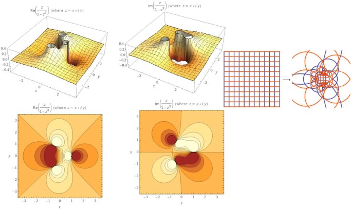

  

  The behavior of solutions of Eq.(3.2), when $\alpha =0.25$, $\beta =1$

Solutions of perturbed Bernoulli’s equation are formulated in the following theorem.

Theorem 3.10

Let λ be analytic and g be an analytic starlike function in ∪. Assume that $\sigma \in \wedge$ is a solution of Bernoulli’s equation

$$ \Theta \bigl[\sigma (\xi )\bigr]= \lambda (\xi )+\epsilon , \quad \epsilon > 0, $$

where $(\Theta [\sigma (\xi ) )^{-1} \in \mathcal{C}$ and

$$ \Re \bigl( \Theta \bigl[\sigma (\xi )\bigr] \bigr)=\Re \biggl((1-\alpha ) \biggl(\frac{\xi }{\sigma (\xi )} \biggr)^{\beta }+\alpha \biggl( \frac{\xi }{\sigma (\xi )} \biggr)^{\beta +1} \sigma '(\xi )-1 \biggr) >0. $$

Then σ is a univalent solution of the Briot–Bouquet equation

$$ \sigma (\xi )+ \frac{\sigma ' (\xi )g(\xi )}{g'(\xi )[\sigma (\xi )+\epsilon ]}= \lambda (\xi ) $$

such that $\Re (\sigma (\xi )+\epsilon )>0$ admitting the structure

$$\begin{aligned} \sigma (\xi )= \Upsilon ^{\epsilon }(\xi ) \biggl( \int _{0}^{\xi }\frac{g' (\tau )\Upsilon (\tau )}{g(\tau )}\,d\tau \biggr)^{-1}- \epsilon , \end{aligned}$$

(3.3)

where

$$ \Upsilon (\xi )= g(\xi ) \exp \biggl( \frac{\int _{0}^{\xi }\frac{g'(\tau )\lambda (\tau )}{g(\tau )}\,d\tau }{\epsilon } \biggr). $$

Proof

Since g is a starlike analytic function in ∪, then

$$ \Re \biggl(\frac{\xi g' (\xi )}{g(\xi )} \biggr)>0, \quad \xi \in \cup . $$

Define a function $Q: \cup \rightarrow \cup$ as follows:

$$ Q(\xi ):= \biggl(\frac{\xi g' (\xi )}{g(\xi )} \biggr) \Theta \bigl[ \sigma (\xi ) \bigr]. $$

Thus, $\Re (Q(\xi ) )>0$. According to [2]-Theorem 3.4j, the Briot–Bouquet equation

$$ \sigma (\xi )+ \frac{\sigma ' (\xi )g(\xi )}{g'(\xi )[\sigma (\xi )+\epsilon ]}= \lambda (\xi ) $$

such that $\Re (\sigma (\xi )+\epsilon )>0$. Since $(\Theta [\sigma (\xi ) )^{-1} \in \mathcal{C}$, then we have

$$ \Re \biggl(Q(\xi )+ 1+ \frac{\xi ( (\Theta [\sigma (\xi ) )^{-1} )'' }{ ( (\Theta [\sigma (\xi ) )^{-1} )'} \biggr) >0. $$

According to [2]-Theorem 3.4k, the solution of the Briot–Bouquet equation is univalent in ∪ taking formula (3.3). □

4 Conclusion

The above study showed a deep investigation of a class of analytic normalized functions in the open unit disk taking Bernoulli’s formula equations. The class was studied previously when $\beta <\alpha \leq 1$ (see [14]). In this effort, we considered $\alpha \leq 1\leq \beta <\infty$. Applications are illustrated to discover the geometric behavior of solutions, not only for the complex Bernoulli’s equations, but for some inequalities as well. The recent work can be studied by suggesting other classes of analytic functions such as meromorphic [17], harmonic, and multivalent classes [18].

References

Ma, W., Minda, D.: A unified treatment of some special classes of univalent functions. In: Li, Z., Ren, F., Yang, L., Zhang, S. (eds.) Proceeding of the Conference on Complex Analysis, pp. 157–169. International Press, Somerville (1994)
Miller, S.S., Mocanu, P.T.: Differential Subordinations: Theory and Applications. CRC Press, Boca Raton (2000)
Wani, L.A., Swaminathan, A.: Starlike and convex functions associated with a nephroid domain. Bull. Malays. Math. Soc. 44(1), 79–104 (2021)
Raducanu, D.: Second Hankel determinant for a class of analytic functions defined by q-derivative operator. An. Ştiinţ. Univ. ‘Ovidius’ Constanţa, Ser. Mat. 27(2), 167–177 (2019)
Ibrahim, R.W.: Geometric process solving a class of analytic functions using q-convolution differential operator. J. Taibah Univ. Sci. 14(1), 670–677 (2020)
Ibrahim, R.W., Elobaid, R.M., Obaiys, S.J.: Symmetric conformable fractional derivative of complex variables. Mathematics 8(3), 363 (2020)
Ibrahim, R.W., Elobaid, R.M., Obaiys, S.J.: A class of quantum Briot-Bouquet differential equations with complex coefficients. Mathematics 8(5), 794 (2020)
Ibrahim, R.W., Darus, M.: On a class of analytic functions associated to a complex domain concerning q-differential-difference operator. Adv. Differ. Equ. 2019(1), 1 (2019)
Murugusundaramoorthy, G., Sokol, J.: On λ-pseudo bi-starlike functions related to some domains. Bull. Transilv. Univ. Braşov Ser. III 12(2), 381–392 (2019)
Raina, R.K., Sokol, J.: On a class of analytic functions governed by subordination. Acta Univ. Sapientiae Math. 11(1), 144–155 (2019)
Ibrahim, R.W., Jahangiri, J.M.: Conformable differential operator generalizes the Briot-Bouquet differential equation in a complex domain. AIMS Math. 4(6), 1582–1595 (2019)
Ibrahim, R.W., Darus, M.: New symmetric differential and integral operators defined in the complex domain. Symmetry 11(7), 906 (2019)
Shanmugam, T.N., Sivasubramanian, S., Srivastava, H.M.: Differential sandwich theorems for certain subclasses of analytic functions involving multiplier transformations. Integral Transforms Spec. Funct. 17(12), 889–899 (2006)
Sivasubramanian, S., Darus, M., Ibrahim, R.W.: On the starlikeness of certain class of analytic functions. Math. Comput. Model. 54(1–2), 112–118 (2011)
Ruscheweyh, S.: Convolutions in Geometric Function Theory. Les Presses De L’Universite De Montreal, Montreal (1982)
Campbell, D.M.: Majorization-subordination theorems for locally univalent functions, II. Can. J. Math. 25(2), 420–425 (1973)
Ibrahim, R.W., Aldawish, I.: Difference formula defined by a new differential symmetric operator for a class of meromorphically multivalent functions. Adv. Differ. Equ. 2021, 281 (2021)
Darus, M., Aldawish, I., Ibrahim, R.W.: Some concavity properties for general integral operators. Bull. Iranian Math. Soc. 41(5), 1085–1092 (2015)
Acknowledgements
Not applicable.
Funding
Author information
Authors and Affiliations
Contributions
All authors contributed equally and significantly in writing this article. All authors read and approved the final manuscript.
Corresponding author
Ethics declarations
Competing interests
The authors declare that they have no competing interests.
Rights and permissions
Open Access This article is licensed under a Creative Commons Attribution 4.0 International License, which permits use, sharing, adaptation, distribution and reproduction in any medium or format, as long as you give appropriate credit to the original author(s) and the source, provide a link to the Creative Commons licence, and indicate if changes were made. The images or other third party material in this article are included in the article’s Creative Commons licence, unless indicated otherwise in a credit line to the material. If material is not included in the article’s Creative Commons licence and your intended use is not permitted by statutory regulation or exceeds the permitted use, you will need to obtain permission directly from the copyright holder. To view a copy of this licence, visit http://creativecommons.org/licenses/by/4.0/.
About this article
Cite this article
Ibrahim, R.W., Aldawish, I. & Baleanu, D. On a geometric study of a class of normalized functions defined by Bernoulli’s formula. Adv Differ Equ 2021, 463 (2021). https://doi.org/10.1186/s13662-021-03622-3
Received:
Accepted:
Published:
DOI: https://doi.org/10.1186/s13662-021-03622-3