A terrorism-based differential game: Nash differential game

Abstract

In this paper, we investigate the problem of combating terrorism by the government, which is one of the most serious problems that direct governments and countries. We formulate the problem and use the Nash approach of a differential game to obtain the optimal strategies for combating terrorism. We study the relationship between each of the government’ strategies and terrorism when the government is on the defensive (reactive), and we study when the government expects terrorist attacks and develops its strategies to combat terrorism. Also, we study the relationship between government activity and its strategies as well as government activity and the strategy of terrorist organizations.

Introduction

Terrorism is defined as the deliberate use of indiscriminate violence in order to achieve political, religious, or ideological objectives. Throughout the world, terrorism has become a major threat. Counter-terrorism requires government initiatives to promote education quality, employment opportunity, social fairness, religious awareness, and security systems. Some mathematical areas, such as operations research, have been used to develop techniques to combat terrorism. In order to prevent terrorist attacks, governments have imposed restrictions on terrorist organizations, such as freezing their assets and launching military invasions to remove the terrorists. Counter-terrorist measures take into account the reactions of terrorists. In this research, we analyze the interaction strategies between the government and terrorist organizations using a differential game technique. Weapons, financial wealth, and technological competence are used to quantify an organization’s power. While the recruitment of terrorists is carried out by existing terrorists, their own activities and government anti-terrorist measures influence the rate of terrorist recruitment. However, the government incurs costs in countering terrorism in addition to limiting terrorist resources and activity. Terrorist organizations, on the other hand, want to maximize their strength in terms of both size and terrorist acts. As a result, this study examines how to assist governments in their fight against terrorism. Notably, the Nash differential game plays a critical role in the fight against terrorism.

Caulkins et al. [1] explored the optimal control of terrorism and global reputation. They concluded that the ability to combat terrorism depends on public opinion, and two water and fire management techniques were compared. The efficiency of water and fire strategies were compared by Caulkins et al. [2]. A differential game which controls the movements of two territories that can be moveable and fixed was introduced by Hsia et al. [3, 4]. They analyzed the question of territorial defense and defined it as a fuzzy differential game, and they introduced a fuzzy control technique to handle this issue. The parametric Nash collative differential games were investigated by Youness et al. [5]. They introduced a parametric examination of this problem, as well as the solvability set and first- and second-kind stability sets. Megahed et al. [6] presented a large-scale differential game problem. They developed a Nash method for resolving this issue. Additionally, they used Nash and min-max zero-sum techniques to find the best control strategy for the fuzzy differential game [7–9]. Nova et al. [10] addressed a terrorism-related differential game. They discussed the Nash and Stackelberg strategies as well as their sensitivity analyses. Roy et al. [11] developed the concept of strategic interdependence between countries for the purpose of deterring terrorism. In a game with multiple stages and incomplete information, they investigated the balance reactions (for defence, R&D, and prevention) to a hypothetical terrorist attack in a two-country context. Megahed [12, 13] used the min-max approach to define the government and international terrorist organization’s (ITO) optimal strategy. He looked at two questions, i.e., – governments and ITO, and showed how important government procedures are in the fight against terrorism. In [14], he also described the Stackelberg differential game involving an E-differentiable function and an E-convex set. Additionally, Megahed in [15] emphasized the importance of the government’s operations in counter-terrorism, and the Stackelberg approach was used to analyze the differential game between the government and terrorists. Arce et al. [16] examined the prevalence of deterrence over preemption when governments can pick between the two approaches or combine them. In [17], they conducted a review of previous uses of game theory to the study of terrorism. Short et al. [18] researched how small violent fringe groups grow into huge, indoctrinated civilizations by modeling radicalization. In [19], they studied the spatiotemporal correlation of terrorist activities by al-Qaeda, the Islamic State of Iraq and Syria (ISIS), and local militants in six geographical locations, and in [20] they used game theory to protect oil and gas infrastructure from terrorism. Lazreg et al. in [21] studied the impulsive Caputo–Fabrizio fractional differential equations in b-metric spaces. Adiguzel et al. [22] discussed the use of Geraghty type hybrid contractions to solve fractional differential equations. Sevinik, Adiguzel et al. [23] looked at how to solve a boundary value problem involving a fractional differential equation. Adiguzel et al. [24] discussed how unique solutions exist for higher-order nonlinear fractional differential equations with multi-point and integral boundary conditions. Nguyen Duc Phuong et al. [25] developed a modified quasi boundary value method for the bi-parabolic equation’s inverse source problem, and semilinear problems involving nonlinear operators of monotone type were studied by In-Sook Kima [26].

Problem formulation

Consider the state variable $Z(t)$ in the differential game, which represents an ITO’s resources that include weapons, financial capital, and a support network. Take another variable state $\kappa (t)$ that describes the operations of the government (All these factors must be taken into account, including the quality of education, employment opportunities, social justice, religious awareness, and security arrangements.) $t\in [ 0,\infty )$. The two participants are the government, which has a nonnegative strategy $\nu _{1}(t)$, and the ITO, which has a nonnegative strategy $\nu _{2}(t)$. The resource stock of the ITO grows in a linear function $G(Z)$, i.e., $G(Z)= r~Z$, $r>0$, and government activity rises in a linear function $B(\kappa )=\xi \kappa$, $\xi > 0$ is the government activity’s rate of growth. Attacking slows the increase of the resource pool because it has a negative impact on the number of terrorists as well as weapons and money resources (for example, due to suicide bombings or terrorists being caught or killed). It is possible that the network of supporters will shrink as a result. The reduction in resource stock growth, on the other hand, is dependent not only on the intensity of the assault $\nu _{2}$, but also on counter-terrorism efforts $\nu _{1}$. The harvest function $h(\nu _{1},\nu _{2})$ represents the influence of the two players’ control variables on resource growth. As a result, the resource stock’s $Z(t)$ dynamics can be stated like this:

$$\begin{aligned}& \frac{d Z}{d t} =r~Z(t)-h(\nu _{1},\nu _{2}), \quad Z(0)=Z_{0}>0, \\& \frac{d \kappa }{d t} =\xi~\kappa + b_{1} \nu _{2}-a_{1} \nu _{1}, \quad \kappa (0)=\kappa _{0} > 0. \end{aligned}$$

The initial terrorist stock is $Z_{0}$, while $\kappa_{0}$ is the initial activities of the government, and $a_{1},b_{1}>0$. Moreover, we assume the following nonnegativity constraints along trajectories $Z(t)$ and $\kappa (t)$.

We assume that the partial derivatives are greater than zero because higher intensity of counter-terrorism efforts and attacks leads to a decline in growth: $\frac{\partial h}{\partial \nu _{1}}>0$, $\frac{\partial h}{\partial \nu _{2}}>0$. The effectiveness of counter-terrorism efforts is dwindling $\frac{\partial ^{2} h}{\partial \nu _{1} \partial \nu _{2}}<0$. Furthermore, a higher attack rate results in disproportionately higher resource losses, i.e., $\frac{\partial ^{2} h}{\partial \nu _{2}^{2} }>0$. Finally, the instruments complement one another, i.e., $\frac{\partial ^{2} h }{\partial \nu _{1} \partial \nu _{2}}>0$. This is financially sound. Because active and visible terrorists are easier to manage than concealed terrorists, this positive relationship suggests that the marginal efficiency of counter-terrorism actions rises as the intensity of terrorist assaults rises. We also suppose that the economic literature’s Inada requirements are met [27].

$$\begin{aligned}& \lim_{\nu _{1}\rightarrow 0}\frac{\partial h}{\partial {\nu _{1}}} = \infty ,\qquad \lim _{\nu _{1}\rightarrow \infty } \frac{\partial h}{\partial {\nu _{1}}}=0, \end{aligned}$$

(1)

$$\begin{aligned}& \lim_{\nu _{2}\rightarrow 0}\frac{\partial h}{\partial {\nu _{2}}} = 0,\qquad \lim _{\nu _{2}\rightarrow \infty } \frac{\partial h}{\partial {\nu _{2}}}=\infty . \end{aligned}$$

(2)

This ensures that the best strategies are not negative, $\nu _{1}\geq 0$ and $\nu _{2}\geq 0$.

Player 1 (Government) derives benefit from its actions $\kappa (t)$, harvest function $h(\nu _{1},\nu _{2} )$, the depletion of terrorist resources $(-c~Z(t))$. However, inefficiencies due to the ITO’s size $(-k~\nu _{2})$, terrorist activities, and their own counter-terrorism measures all add up to costs. $(-\alpha _{1} \nu _{1})$ The government’s ongoing payment at time intervals of $[0,\infty )$ (the government’s goal) is

$$ \max_{\nu _{1 }}J_{1}= \int _{0}^{\infty }e^{-\zeta _{1}t} \bigl[ \omega _{1}~h(\nu _{1},\nu _{2})+ q~\kappa (t)-c~Z-k~\nu _{2} - \alpha _{1} \nu _{1} \bigr]\,dt, $$

(3)

where $\omega _{1}, c, k, q$, and $\alpha _{1} > 0$

The utility of the second player (ITO) is derived from the stock of resources. $(\sigma _{1} Z)$ as well as terrorist acts $(-\gamma _{1} \kappa (t))$ at a high level $(\beta _{1} \nu _{2} )$, then the ITO’s running payout (its goal) is to maximize the following problem’s payoff:

$$ \max_{\nu _{2} } J_{2}= \int _{0}^{\infty }e^{-\zeta _{2}t} \bigl[ \sigma _{1} Z(t)+\beta _{1} \nu _{2}-\gamma _{1} \kappa (t) \bigr]\,dt, $$

(4)

where $\sigma _{1}$, $\beta _{1}$, and $\gamma _{1} >0$

It is expected that the declining rates $\zeta _{i}$, $i=1,2$, are greater than r and ξ growth and activity rates:

$$ \zeta _{i}> r, \qquad \zeta _{i}> \xi \quad {\text{for } i=1,2}. $$

(5)

The Nash equilibria are calculated in this study. The approach for solving the problem is based on Pontryagin’s maximum principle [9].

Nash differential game

A continuous differential game with N players is a Nash differential game. Ordinary differential equations regulate how the game’s state is evaluated throughout time. Each participant affects the outcome of the game by selecting an acceptable strategy. The cost of a player is determined by all players’ strategies and the state’s related evaluation. Differential equations are used to express information about the players, such as the target set, all players’ cost functions, and the current space. It is assumed that each player’s opponents are rational and that each player employs an optimal strategy, in which each player seeks to maximize his own gain. The Nash equilibrium notion essentially states that if one person tries to change his approach unilaterally, he will not be able to better his own optimization.

Definition 1

If the cost functions for players $1,2,\ldots,N$ are $J_{1}(\nu _{1}, \nu _{2},\ldots, \nu _{N}),\ldots,J_{n}(\nu _{1},\nu _{2}, \ldots, \nu _{N})$, then $(\nu _{1}^{*},\nu _{2}^{*},\ldots,\nu _{N}^{*})$ is said to be a Nash equilibrium strategy if, for $i=1,2,\ldots,N$,

$$ J_{i}\bigl(\nu _{1}^{*},\ldots,\nu _{i},\ldots,\nu _{n}^{*}\bigr)\geq J_{i}\bigl(\nu _{1}^{*},\ldots, \nu _{i}^{*},\ldots,\nu _{N}^{*}\bigr). $$

(6)

The Nash equilibrium solutions for two players, the government and the ITO, are investigated in this research.

Nash equilibrium

Take the next problem:

$$ \left. \begin{aligned} &\max_{\nu _{1}}J_{1}= \int _{0}^{\infty }e^{-\zeta _{1}t} \bigl[ \omega _{1}~h(\nu _{1},\nu _{2})+q \kappa -c Z-k \nu _{2}-\alpha _{1} \nu _{1} \bigr]\,dt, \\ &\max_{\nu _{2} } J_{2}= \int _{0}^{\infty }e^{-\zeta _{2}t} [ \sigma _{1}~Z+\beta _{1} \nu _{2} -\gamma _{1}~\kappa ]\,dt, \\ &\frac{d Z}{d t}=r~Z(t)-h(\nu _{1},\nu _{2}),\qquad Z(0)=Z_{0}>0 ,\quad Z \geq 0, \\ &\frac{d \kappa }{d t}=\xi~\kappa + b_{1} \nu _{2} - a_{1} \nu _{1},\qquad \kappa (0)=\kappa _{0}>0 , \quad \kappa (t) \geq 0 . \end{aligned} \right\} $$

(7)

The Hamiltonian government’s $H_{1}$ function is defined by

$$ \begin{aligned}H_{1}={}&\omega _{1}~ h(\nu _{1}, \nu _{2}) + q~\kappa (t)- c~Z(t)-k~\nu _{2}-\alpha _{1} \nu _{1}+\chi _{1}(t)~\bigl( r~Z(t)-h(\nu _{1}, \nu _{2})\bigr) \\ &{}+ \chi _{2}(t)~\bigl(\xi~\kappa (t) + b_{1} \nu _{2} - a_{1} \nu _{1}\bigr), \end{aligned} $$

where $\chi _{1}$ and $\chi _{2}$ are called the costate variables or the adjoint variables associated with the state variables $Z(t)$ and $\kappa (t)$ for ITO and the government, respectively.

The ITO’s Hamiltonian is defined as

$$\begin{aligned} H_{2} =&\sigma _{1} Z(t)+\beta _{1} \nu _{2} (t)-\gamma _{1} \kappa (t)+ \Psi _{1}(t) \bigl(r Z(t)-h(\nu _{1}, \nu _{2})\bigr) \\ &{}+\Psi _{2}(t) \bigl(\xi \kappa (t)+ b_{1} \nu _{2}- a_{1} \nu _{1}\bigr), \end{aligned}$$

where $\Psi _{1}$ and $\Psi _{2}$ are the costate variables or adjoint variables for ITO and government, respectively, and are related with the state variables $Z(t)$ and $\kappa (t)$.

The government’s and ITO’s best tactics must maximize the Hamiltonians $H_{1}$ and $H_{2}$; thus, the first-order conditions are obtained:

$$ \frac{\partial H_{1}}{\partial \nu _{1}}=(\omega _{1}-\chi _{1}) \frac{\partial h}{\partial {\nu _{1}}}-\alpha _{1}-a_{1} \chi _{2}=0 \quad \Rightarrow\quad \nu _{1}^{*}=\nu _{1}^{*}( \nu _{2}, \chi _{1}, \chi _{2} ) $$

(8)

and

$$ \frac{\partial H_{2}}{\partial \nu _{2}}=\beta _{1}-\Psi _{1} { \frac{\partial h}{\partial {\nu _{2}}}}+b_{1}\Psi _{2}=0 \quad \Rightarrow\quad \nu _{2}^{*}=\nu _{2}^{*}(\nu _{1, \Psi _{1},\Psi _{2}}). $$

(9)

$\chi _{1}$, $\chi _{2}$, $\Psi _{1}$, and $\Psi _{2}$ are adjoint variables that satisfy the differential equations

$$ \begin{aligned} &\frac{{d\chi _{1}}}{dt}=\zeta _{1}\chi _{1}- \frac{\partial H_{1}}{\partial Z}=(\zeta _{1}-r)\chi _{1}+c, \\ &\frac{d\chi _{2}}{dt}=\zeta _{1}\chi _{2}- \frac{\partial H_{1}}{\partial \kappa }=(\zeta _{1}-\xi )\chi _{2}-q, \\ &\frac{d\Psi _{1}}{dt}=\zeta _{2}\Psi _{1}- \frac{\partial H_{2}}{\partial Z}=(\zeta _{2}-r)\Psi _{1}-\sigma _{1}, \\ &\frac{d\Psi _{2}}{dt}=\zeta _{2}\Psi _{2}- \frac{\partial H_{2}}{\partial \kappa }=(\zeta _{2}-\xi )\Psi _{2}+ \gamma _{1}. \end{aligned} $$

(10)

The conditions that limit transversality are as follows:

$$ \begin{aligned} &\lim_{t\to \infty } \int _{0}^{\infty }e^{-(\zeta _{1}-r)t} Z(t) \chi _{1}(t)\,dt =0, \\ &\lim_{t\to \infty } \int _{0}^{\infty }e^{-(\zeta _{1}-\xi )t} \kappa (t) \chi _{2}(t)\,dt =0, \\ &\lim_{t\to \infty } \int _{0}^{\infty }e^{-(\zeta _{2}-r)t} Z(t) \Psi _{1}(t)\,dt =0, \\ &\lim_{t\to \infty } \int _{0}^{\infty }e^{-(\zeta _{2}-\xi )t} \kappa (t) \Psi _{2}(t)\,dt =0. \end{aligned} $$

(11)

The adjoint equations’ solutions (10) are

$$ \begin{aligned} &\chi _{1}= \biggl(\chi _{10}+ \frac{c}{\zeta _{1}-r} \biggr)e^{(\zeta _{1}-r)t}- \frac{c}{\zeta _{1}-r}, \\ &\chi _{2}= \biggl(\chi _{20}-\frac{q}{\zeta _{1}-\xi } \biggr)e^{( \zeta _{1}-\xi )t}+\frac{q}{\zeta _{1}-\xi }, \\ &\Psi _{1}= \biggl(\Psi _{10}-\frac{\sigma _{1}}{\zeta _{2}-r} \biggr)e^{( \zeta _{2}-r)t}+\frac{\sigma _{1}}{\zeta _{2}-r}, \\ &\Psi _{2}= \biggl(\Psi _{20}+\frac{\gamma _{1}}{\zeta _{2}-\xi } \biggr)e^{( \zeta _{2}-\xi )t}-\frac{\gamma _{1}}{\zeta _{2}-\xi }. \end{aligned} $$

(12)

The adjoint variables diverge to ±∞ according to condition (5), violating the terms of the transversality, unless the values in the steady state are constant

$$ \begin{aligned} &\chi _{1}=\chi _{10}=- \frac{c}{\zeta _{1}-r},\qquad \chi _{2}=\chi _{20}= \frac{q}{\zeta _{1}-\xi }, \\ &\Psi _{1}=\Psi _{10}=\frac{\sigma _{1}}{\zeta _{2}-r},\qquad \Psi _{2}= \Psi _{20}=-\frac{\gamma _{1}}{\zeta _{2}-\xi }. \end{aligned} $$

(13)

With respect to the optimal strategies $\nu_{1}$ and $\nu_{2}$, the Hamiltonians $H_{1}$ and $H_{2}$ are concave, according to (13), where the harvest function is defined as follows:

$$ h(\nu _{1},\nu _{2})=\nu _{1}^{\tau _{1}}\nu _{2}^{\varrho },\quad \varrho >1, 0< \tau _{1} < 1. $$

Proposition 1

The Nash problem’s best strategies can be found in

$$ \begin{aligned} &\nu _{1}= \biggl( \frac{\beta _{1} + b_{1} \Psi _{2}}{\varrho \Psi _{1}} \biggr)^{\frac{\varrho }{\tau _{1} +\varrho -1}} \biggl( \frac{\alpha _{1}+a_{1} \chi _{2}}{\tau _{1} (\omega _{1}-\chi _{1})} \biggr)^{\frac{1-\varrho }{\tau _{1}+\varrho -1}}, \\ &\nu _{2}= \biggl(\frac{\beta _{1}+b_{1} \Psi _{2}}{\varrho \Psi _{1}} \biggr)^{\frac{1-\tau _{1}}{\tau _{1}+\varrho -1}} \biggl( \frac{\alpha _{1}+a_{1} \chi _{2}}{\tau _{1} (\omega _{1}-\chi _{1})} \biggr)^{\frac{\tau _{1}}{\tau _{1}+\varrho -1}}, \\ & h(\nu _{1},\nu _{2})= \biggl( \frac{\beta _{1}+ b_{1} \Psi _{2}}{\varrho \Psi _{1}} \biggr)^{\frac{\varrho }{\tau _{1}+\varrho -1}} \biggl( \frac{\alpha _{1}+a_{1} \chi _{2}}{\tau _{1} (\omega _{1}-\chi _{1})} \biggr)^{\frac{\tau _{1}}{\tau _{1}+\varrho -1}}. \end{aligned} $$

(14)

Proof

From the necessary conditions

$$\begin{aligned}& \frac{\partial H_{1}}{\partial \nu _{1}}=(\omega _{1}-\chi _{1}) \frac{\partial h}{\partial {\nu _{1}}}-\alpha _{1}-a_{1}\chi _{2}=0, \\& \frac{\partial H_{2}}{\partial \nu _{2}}=\beta _{1}-\Psi _{1} \frac{\partial h}{\partial {\nu _{2}}}+ b_{1} \Psi _{2}=0; \end{aligned}$$

then

$$ \frac{\partial {h}}{\partial {\nu _{1}}}= \frac{\alpha _{1}+ a_{1}\chi _{2}}{\omega _{1}-\chi _{1}},\qquad \frac{\partial h}{\partial \nu _{2}}= \frac{\beta _{1}+b_{1}\Psi _{2}}{\Psi _{1}}. $$

(15)

We have obtained the following results from the harvest function $h( \nu _{1},\nu _{2})$:

$$ \frac{\partial {h}}{\partial \nu _{1}} =\tau _{1} \nu _{1}^{\tau _{1}-1} \nu _{2}^{\varrho }= \frac{\alpha _{1}+a_{1}\chi _{2}}{\omega _{1}-\chi _{1}},\qquad \frac{\partial h}{\nu _{2}}= \varrho \nu _{1}^{\tau _{1}}\nu _{2}^{ \varrho -1}= \frac{\beta _{1}+ b_{1}\Psi _{2}}{\Psi _{1}}; $$

thus,

$$\begin{aligned}& \nu _{1}= \biggl( \frac{\alpha _{1}+a_{1}\chi _{2}}{\tau _{1}(\omega _{1}-\chi _{1})} \biggr)^{\frac{1}{\tau _{1}-1}}\nu _{2}^{\frac{\varrho }{1-\tau _{1}}}, \end{aligned}$$

(16)

$$\begin{aligned}& \nu _{2}= \biggl(\frac{\beta _{1}+ b_{1}\Psi _{2}}{\varrho \Psi _{1}} \biggr)^{\frac{1}{\varrho -1}} \nu _{1}^{\frac{\tau _{1}}{1-\varrho }}. \end{aligned}$$

(17)

By solving (16) and (17), we obtain

$$ \begin{aligned} &\nu _{1}= \biggl( \frac{\beta _{1}+b_{1} \Psi _{2}}{\varrho \Psi _{1}} \biggr)^{\frac{\varrho }{\tau _{1}+\varrho -1}} \biggl( \frac{\alpha _{1} + a_{1} \chi _{2}}{\tau _{1} (\omega _{1}-\chi _{1})} \biggr)^{\frac{1-\varrho }{\tau _{1}+\varrho -1}}, \\ &\nu _{2}= \biggl( \frac{\beta _{1} + b_{1} \Psi _{2}}{\varrho \Psi _{1}} \biggr)^{\frac{1-\tau _{1}}{\tau _{1}+\varrho -1}} \biggl( \frac{\alpha _{1}+ a_{1} \chi _{2}}{\tau _{1} (\omega _{1}-\chi _{1})} \biggr)^{\frac{\tau _{1}}{\tau _{1}+\varrho -1}}, \\ &h(\nu _{1},\nu _{2})= \biggl( \frac{\beta _{1} + b_{1} \Psi _{2}}{\varrho \Psi _{1}} \biggr)^{\frac{\varrho }{\tau _{1}+\varrho -1}} \biggl( \frac{\alpha _{1}+a_{1} \chi _{2}}{\tau _{1} (\omega _{1}-\chi _{1})} \biggr)^{\frac{\tau _{1}}{\tau _{1}+\varrho -1}}. \end{aligned} $$

(18)

 □

Remark

• 1. In (16), since $\varrho > 1$; $0 < \tau _{1} < 1$, then the power of $\nu _{2}$ is greater than 1 ($\frac{\varrho }{1-\tau _{1}}>1$)). This relation shows that the government is more aggressive when ITO increases their attacks and when the harvest function increases, as shown in Fig. 1. More discussion: Equation (16) showed the relationship between the strategy of the terrorist organization and the strategy of the government. We obtained this relationship from the condition $\frac{\partial H_{1}}{\partial \nu _{1}}=0$. The government had neglected for short time the fight against terrorist organizations, after that it became aware and began to take measures and developed its strategies, this was shown in Fig. 1. We found that the government had played its role and taken control of the situation; for this, the activity of terrorist organizations stopped at a specific level, which was some light work. Also, we note that the government’s actions were a reaction to the terrorist organizations, but the reaction continued until the government took complete control of the situation.

  Figure 1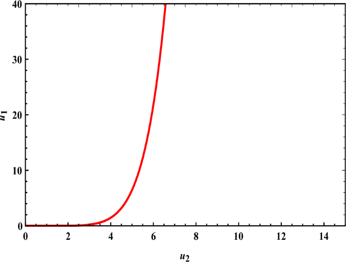

  

  The government is more aggressive when the ITO increases their attacks

• 2. In (17), since $\varrho > 1$, $0 < \tau _{1} < 1$, then the power of $\xi _{1}$ is less than 1, ($\frac{\tau _{1}}{1-\varrho }<1$) an increase in counter-terror measures leads to a more cautious behavior by the terrorists and a lower harvest function, as shown in Fig. 2. Also, equation (17) showed the relationship between the strategies of terrorist organizations and the strategies of the government, which we obtained from the condition $\frac{\partial H_{2}}{\partial \nu _{2}}=0$. Through this relationship, we noticed that when the government neglected the fight against terrorism, the organizations developed themselves and spread widely, this is clear from Fig. 2$\nu _{1}\rightarrow 0$ as $\nu _{2}\rightarrow \infty$; and when the government fulfilled its duty towards this problem, the activities of the organizations began to decline, and the government did not stop until it took control of the situation, which put things back in order, restricted terrorism, and the situation became stable $\nu _{1}\rightarrow \infty$ as $\nu _{2}\rightarrow 0$.

  Figure 2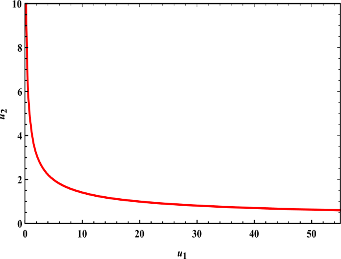

  

  An increase in counter-terror measures makes the terrorists more cautious

Lemma 1

For a constant harvest and constant strategies $h(\nu _{1}, \nu _{2})$ and $\nu _{1}$, $\nu _{2}$ for the governments’ objective $J_{1}$ and ITO’ objective $J_{2}$ are

$$\begin{aligned}& J_{1}=\frac{\omega _{1} h}{\zeta _{1}}+\frac{q}{\zeta _{1}-\xi } \biggl(\kappa _{0}-\frac{a_{1} \nu _{1}-b_{1} \nu _{2}}{\xi } \biggr)+ \frac{a _{1}\nu _{1}-b_{1} \nu _{2}}{\xi \zeta _{1}}- \frac{c}{\zeta _{1}-r} \biggl( Z_{0}-\frac{h}{r} \biggr)- \frac{c h}{r\zeta _{1}}, \\& J_{2}=\frac{\sigma _{1}}{\zeta _{2}-r} \biggl(Z_{0}-\frac{h}{r} \biggr)+ \frac{\sigma _{1} h}{r\zeta _{2}}+ \frac{\beta _{1} \nu _{2}}{\zeta _{2}}- \frac{\gamma _{1}}{\zeta _{2}-\xi } \biggl(\kappa _{0}- \frac{a_{1} \nu _{1}-b_{1} \nu _{2}}{\xi } \biggr)- \frac{\gamma _{1} (a_{1} \nu _{1}-b_{1} \nu _{2})}{\xi \zeta _{2}}. \end{aligned}$$

Proof

The differential equation’s solution $\frac{d \kappa }{d t}=\xi \kappa + b_{1} \nu _{2}-a_{1} \nu _{1}$ is

$$ \kappa (t)= \biggl(\kappa _{0}- \frac{a_{1} \nu _{1}-b_{1} \nu _{2}}{\xi } \biggr)e^{\xi t}+ \frac{a_{1} \nu _{1}-b_{1} \nu _{2}}{\xi }. $$

(19)

From (16) in (19), we have

$$ \kappa (t)=\kappa _{0} e^{\xi t}-\frac{b_{1}}{\xi } \bigl(1-e^{\xi t}\bigr) \nu _{2} + \frac{a_{1}}{\xi } \bigl( \bigl(1-e^{\xi t}\bigr) \bigr) \biggl( \frac{\alpha _{1}+a_{1}\chi _{2}}{\tau _{1}(\omega _{1}-\chi _{1})} \biggr)^{\frac{1}{\tau _{1}-1}}\nu _{2}^{\frac{\varrho }{1-\tau _{1}}}, $$

(20)

and from (17) in (19), we have

$$ \kappa (t)= \kappa _{0}e^{\xi t}+\frac{a_{1}}{\xi }\bigl(1-e^{\xi t}\bigr) \nu _{1} -\frac{b_{1}}{\xi } \bigl(1+ e^{\xi t} \bigr) \biggl( \frac{\beta _{1} + b_{1}\Psi _{2}}{\varrho \Psi _{1}} \biggr)^{\frac{1}{1-\varrho }}\nu _{1}^{\frac{\tau _{1}}{1-\varrho }}, $$

(21)

and the differential equation’s solution $\frac{d Z}{d t} = r Z-h( \nu _{1},\nu _{2})$ is

$$ Z(t)= \biggl(Z_{0}-\frac{h}{r} \biggr)e^{r t}+ \frac{h}{r}. $$

(22)

In the government objective $J_{1}$ and the ITO objective $J_{2}$, from (19) and (22),

$$\begin{aligned} J_{1} =& \int _{0}^{\infty }e^{-\zeta _{1}t} \biggl[\omega _{1}~h + q~\biggl(\kappa _{0}-\frac{a_{1} \nu _{1}-b_{1} \nu _{2}}{\xi } \biggr)~e^{ \xi t}+\frac{q~(~a_{1}\nu _{1}-b_{1} \nu _{2})}{\xi } \\ &{}-c \biggl(Z_{0}- \frac{h}{r} \biggr)~e^{r t}- \frac{c h}{r}-k \nu _{2}-\alpha _{1} \nu _{1} \biggr]\,dt \\ =&\frac{\omega _{1} h}{\zeta _{1}}+\frac{q}{\zeta _{1}-\xi } \biggl( \kappa _{0}- \frac{a_{1} \nu _{1}-b_{1} \nu _{2}}{\xi } \biggr)+ \frac{q~(a_{1} \nu _{1}-b_{1}\nu _{2})}{\xi~\zeta _{1}} \\ &{}- \frac{c}{\zeta _{1}-r} \biggl(Z_{0}-\frac{h}{r} \biggr)- \frac{c~h}{r~\zeta _{1}}-\frac{ k~\nu _{2}}{\zeta _{1}}- \frac{\alpha _{1} \nu _{1}}{\zeta _{1}} \end{aligned}$$

and

$$\begin{aligned} J_{2} =& \int _{0}^{\infty }e^{-\zeta _{2}t} \biggl[\sigma _{1} \biggl( Z_{0}- \frac{ h}{r} \biggr)~e^{rt}+\frac{\sigma _{1}~h}{r}-\gamma _{1} \biggl( \kappa _{0}-\frac{a_{1}\nu _{1}-b_{1}\nu _{2}}{\xi } \biggr)e^{\xi t} \\ &{}+ \frac{\gamma _{1}~(a~\nu _{1}-b_{1} \nu _{2})}{\xi }+\beta _{1} \nu _{2} \biggr]\,dt \\ =&\frac{\sigma _{1}}{\zeta _{2}-r} \biggl(\kappa _{0}-\frac{ h}{r} \biggr)+ \frac{\sigma _{1}~h}{r~\zeta _{2}}- \frac{\gamma _{1}}{\zeta _{2}-\xi } \biggl(\kappa _{0}- \frac{a_{1} \nu _{1}-b_{1} \nu _{2}}{\xi } \biggr) \\ &{}- \frac{\gamma _{1}~(a_{1} \nu _{1}-b_{1}\nu _{2})}{\xi~\zeta _{2}}+ \frac{\beta _{1} \nu _{2}}{\zeta _{2}}, \end{aligned}$$

where $\nu _{1}$, $\nu _{2}$ as well as $h(\nu _{1},\nu _{2})$ are given in(18). □

Remark

• 1. Equation (20) represents the relationship between government activity $\kappa (t)$ and the strategies of the terrorist organization $\nu _{2}$. When $\nu _{2}\rightarrow 0$, the government had a clear activity, and the relationship became increasing until the maximum value. After that the relationship became decreasing as the organizations increased their activity and developed their strategies, which affected the government that abandoned some of its duties until the organization took control of the state’s capabilities as shown in Fig. 3.

  Figure 3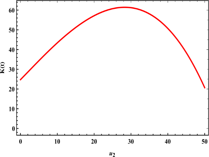

  

  The government’ activities are decreasing with (ITO) increasing their attacks

• 2. Equation (21) represents the relationship between the government’s activity $\kappa (t)$ and its strategies $\nu _{1}$. When the strategies were weak, this reflected on the government’s performance, which also became weak; when the government developed its strategy, this led to an increase in its activity, and this activity continued with the development of government strategies until it reached to the stability, this is evident in Fig. 4.

  Figure 4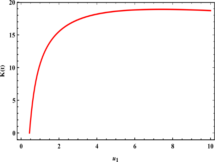

  

  The government’ activity increase with the development of its strategies until the stability position

Conclusions

We studied the problem of combating terrorism, so we formulated the problem and used the Nash approach of a differential game for obtaining the optimal strategies for combating terrorism, and we obtained several relationships, which are the relationship between the strategies of the government and terrorist organizations when the government is in a state of reaction and vice versa. We saw that the government is more violent when it is attacked by terrorist organizations. Likewise, when the government neglects its role, the terrorist organizations control the situation, this is clear in Fig. 1 and Fig. 2. Also, we deduced the relationship between the government’s activity and strategies, as well as the strategies of terrorist organizations, this is evident in Figs. 3 and 4.

References

Caulkins, J.P., Feichtinger, G., Grass, D., Tragler, G.: Optimal control of terrorism and global reputation: a case study with novel threshold behavior. Oper. Res. Lett. 37(6), 387–391 (2009)
Caulkins, J.P., Feichtinger, G., Grass, D., Tragler, G.: Optimizing counter-terror operations: should one fight with “fire” or “water”? Comput. Oper. Res. 35(6), 1874–1885 (2008)
Hsia, K.H., Hsie, J.G.: A first approach to fuzzy differential game problem: guarding territory. Fuzzy Sets Syst. 55(2), 157–167 (1993)
Hung, I.C., Hisa, K.H., Chen, L.W.: Fuzzy differential game of guarding a movable territory. Inf. Sci. 91(1–2), 113–131 (1993)
Youness, E., Hughes, J.B., El-kholy, N.: Parametric Nash collative differential games. Math. Comput. Model. 26(2), 97–105 (1997)
Youness, E., Megahed, A.A.E.-M.: A study on large scale continuous differential games. Bull. Calcutta Math. Soc. 94(5), 359–368 (2002)
Youness, E., Megahed, A.A.E.-M.: A study on fuzzy differential game. Le Matematche LVI(Fasc. I), 97–107 (2001)
Hegazy, S., Megahed, A.A.E.-M., Youness, E., Elbanna, A.: Min-max zero-sum two persons fuzzy continuous differential games. Int. J. Appl. Mech. 21(1), 1–16 (2008)
Megahed, A.A.E.-M., Hegazy, S.: Min-max zero two persons continuous differential game with fuzzy control. Asian J. Curr. Eng. Maths 2(2), 86–98 (2013)
Nova, A.J., Feichtinger, G., Leitmann, G.: A differential game related to terrorism: Nash and Stackelberg strategies. J. Optim. Theory Appl. 144(3), 533–555 (2010)
Roy, A., Aliyas, J.: Paul terrorism deterrence in a two country framework: strategic interactions between R&D, defense and pre-emption. Ann. Oper. Res. 211(1), 399–432 (2013)
Megahed, A.A.E.-M.: A differential game related to terrorism: Min-Max Zero-Sum two persons differential game. Neural Comput. Appl. 30(3), 865–870 (2018)
Megahed, A.A.E.-M.: The development of a differential game related to terrorism: Min-Max differential game. J. Egypt. Math. Soc. 25(3), 306–312 (2017)
Megahed, A.A.E.-M.: A differential game related to terrorism: Stackelberg differential game of E-differentiable and E-convex function. Eur. J. Pure Appl. Math. 12(2), 654–668 (2019)
Megahed, A.A.E.-M.: The Stackelberg differential game for counter-terrorism. Qual. Quant. 53(1), 207–220 (2019)
Arce, G.D., Sandler, T.: Counterterrorism: a game-theoretic analysis. J. Confl. Resolut. 40(2), 183–200 (2005)
Sandler, T., Daniel, A.G.: Terrorism: a game-theoretic approach. In: Handbook of Defense Economics, vol. 2, pp. 775–813. Elsevier, Amsterdam (2007)
Short, B.M., Scott, M., D’Orsogna, M.R.: Modeling radicalization: how small violent fringe sects develop into large indoctrinated societies. R. Soc. Open Sci. 4(8), 170678 (2017)
Yao-Li, C., Noam, B., D’Orsogna, M.R.: Local alliances and rivalries shape near-repeat terror activity of al-Qaeda, ISIS and insurgents. Proc. Natl. Acad. Sci. USA 116(42), 20898–20903 (2019)
Rezazadeh, A., Talarico, L., Reniers, G., Cozzani, V., Zhang, L.: Applying game theory for securing oil and gas pipelines against terrorism. Reliab. Eng. Syst. Saf. 191(C), 106–140 (2019)
Jamal, E.L., Saïd, A., Mouffak, B., Erdal, K.: Impulsive Caputo–Fabrizio fractional differential equations in b-metric spaces. Open Math. 19, 363–372 (2021)
Rezan, S.A., Ümit, A., Erdal, K., Inci, E.: On the solutions of fractional differential equations via Geraghty type hybrid contractions. Appl. Comput. Math. 20(2), 313–333 (2021)
Rezan, S.A., Ümit, A., Erdal, K., Inci, E.: On the solution of a boundary value problem associated with a fractional differential equation. Math. Methods Appl. Sci., 1–12 (2020)
Adiguzel, S.R., Aksoy, U., Karapinar, E., Erhan, M.I.: Uniqueness of solution for higher-order nonlinear fractional differential equations with multi-point and integral boundary conditions. Rev. R. Acad. Cienc. Exactas Fís. Nat., Ser. A Mat. 115, 155 (2021)
Phuong, N.D., Luc, H.N., Long, D.L.: Modified quasi boundary value method for inverse source problem of the bi-parabolic equation. Adv. Theory Nonlinear Anal. Appl. 4(3), 132–142 (2020)
In-Sook, K.: Semilinear problems involving nonlinear operators of monotone type. Results Nonlinear Anal. 2(1), 25–35 (2019)
Ken-ichi, I.: On a two-sector model of economic growth: comments and a generalization. In: Review of Economic Studies, vol. 30, pp. 119–127. Oxford University Press, London (1963)
Acknowledgements
I’d like to thank my professors at Suez Canal University in Ismailia, Egypt (Faculty of Computers and Informatics).
Funding
There was no funding available.
Author information
Authors and Affiliations
Contributions
All authors contributed to the manuscript writing, and they all read and approved the final version.
Corresponding author
Ethics declarations
Competing interests
The author declares that they have no competing interests.
Rights and permissions
Open Access This article is licensed under a Creative Commons Attribution 4.0 International License, which permits use, sharing, adaptation, distribution and reproduction in any medium or format, as long as you give appropriate credit to the original author(s) and the source, provide a link to the Creative Commons licence, and indicate if changes were made. The images or other third party material in this article are included in the article’s Creative Commons licence, unless indicated otherwise in a credit line to the material. If material is not included in the article’s Creative Commons licence and your intended use is not permitted by statutory regulation or exceeds the permitted use, you will need to obtain permission directly from the copyright holder. To view a copy of this licence, visit http://creativecommons.org/licenses/by/4.0/.
About this article
Cite this article
Megahed, A.EM.A. A terrorism-based differential game: Nash differential game. Adv Differ Equ 2021, 483 (2021). https://doi.org/10.1186/s13662-021-03635-y
Received:
Accepted:
Published:
DOI: https://doi.org/10.1186/s13662-021-03635-y