
Theory and Modern Applications

Dynamics of a stochastic population model with Allee effects under regime switching

Abstract

A stochastic single-species model with Allee effects under regime switching is developed and detected in the present study. First, extinction and persistence of the model are dissected. Subsequently, sufficient criteria are offered to ensure that the model possesses a unique ergodic stationary distribution. Finally, the theoretical outcomes are employed to evaluate the evolution of the African wild dog (Lycaon pictus) in Africa, and some significant functions of stochastic perturbations are exposed.

1 Introduction

The Allee effect, which is depicted by a relationship between the per capita growth rate and the population size, is a universal biological phenomenon [2, 11, 14]. Allee effects happen while populations rely on cooperation or aggregation to hunt, to prevent capture, or to bring up their young [11, 14]. For instance, the African wild dogs usually form cooperative groups to hunt [4], suricate (Suricata suricatta) and Pacific salmon (Oncorhynchus spp.) form groups to prevent capture [6, 20]. The significance of Allee effects has been admitted in a lot of biological subjects (for example, eco-epidemiology [8], biological invasions [22], and population ecology [7]), and numerous mathematical frameworks have been put forward to dissect the role of Allee effects (see, e.g., [5, 11, 14, 21]). Especially, Takeuchi [21] took advantage of the following equation to test the impacts of Allee effects on the evolution of a population:

$$ \frac{\mathrm{d}\varPsi }{\mathrm{d}t}=\varPsi \biggl[r+ \frac{\mu \varPsi }{1+\lambda \varPsi } - \frac{\varPsi ^{2}}{1+\lambda \varPsi } \biggr], $$
(1)

where \(\varPsi =\varPsi (t)\) means the population size; r indicates the intrinsic growth rate; \(\mu >0\) is the Allee threshold under which the population will become extinct; \(\lambda >0\) depicts the environmental carrying capacity.

All species in natural environments undulate in an essentially random way, and randomness brings a hazard of extinction [19]. Commonly, puny undulations and medium undulations are two classes of usual undulations in the environments [23]. We first appraise the former. Several authors (see, e.g., [1, 9, 10, 1517]) have proffered that the puny undulations often act on the parameters in a system, and one could take advantage of the white noise to approximately depict the puny undulations. In this way, in model (1)

$$ r\rightarrow r+\eta _{1} \dot{\xi _{1}}(t),\qquad \mu \rightarrow \mu + \eta _{2} \dot{\xi _{2}}(t), $$

and accordingly,

$$ \mathrm{d}\varPsi =\varPsi \biggl[r+\frac{\mu \varPsi }{1+\lambda \varPsi }- \frac{\varPsi ^{2}}{1+\lambda \varPsi } \biggr]\,\mathrm{d}t+\eta _{1} \varPsi \,\mathrm{d}\xi _{1}(t)+\frac{\eta _{2}\varPsi ^{2}}{1+\lambda \varPsi } \,\mathrm{d}\xi _{2}(t), $$
(2)

where \(\eta _{i}^{2}\) means the intensity of the white noise, \(\{\xi (t)\}_{t\geq 0}=\{(\xi _{1}(t), \xi _{2}(t))\}_{t\geq 0}\) indicates a Wiener process defined on a complete probability space \((\varOmega , {\{\mathcal{F}_{t}}\}_{t\geq 0}, \mathrm{P})\) which obeys the usual conditions.

Next we appraise the medium undulations (for instance, the medium variations of rainfall and temperature) which are often encountered by the species. When these medium undulations emerge, the parameter values in a system often jump. For instance, Choristoneura fumiferana (Clemens) reproduces 50% more eggs at 25C than at 15C [3]. These medium undulations cannot be portrayed by (2) [12, 1517]. Mathematically, one may employ a finite-state Markov chain to portray these medium undulations [12, 13, 1517]. Denote by \(\theta =\theta (t)\) a right-continuous irreducible Markov chain which is independent of \(\{\xi (t)\}_{t\geq 0}\). Then we can deduce from Eq. (2) that

$$ \mathrm{d}\varPsi =\varPsi \biggl[r(\theta )+ \frac{\mu (\theta )\varPsi }{1+\lambda (\theta )\varPsi } - \frac{\varPsi ^{2}}{1+\lambda (\theta )\varPsi } \biggr]\,\mathrm{d}t+\eta _{1}( \theta )\varPsi \,\mathrm{d}\xi _{1}(t) + \frac{\eta _{2}(\theta )\varPsi ^{2}}{1+\lambda (\theta )\varPsi } \,\mathrm{d}\xi _{2}(t). $$
(3)

During recent decades, there has been growing interest in extinction, persistence, and stability of population models [23]. However, little research has been conducted to appraise these behaviors of (2) and (3). The present study detects these behaviors of (2): we first dissect the extinction and persistence of model (2) in Sect. 2, and then offer sufficient criteria to ensure that model (3) possesses a unique ergodic stationary distribution (UESD) in Sect. 3; in Sect. 4, we make use of the theoretical outcomes to evaluate the evolution of the African wild dog (Lycaon pictus) in Africa and expose some significant functions of puny undulations and medium undulations.

2 Extinction and permanence

Let \(\varTheta =\{1,\ldots,N\}\) and \(\varGamma =(\gamma _{mj})_{N\times N}\) mean the state space and the generator of \(\theta (t)\), respectively, i.e.,

$$ P\bigl\{ \theta (t+\Delta t)=j|\theta (t)=m\bigr\} = \textstyle\begin{cases} \gamma _{mj}\Delta t+o(\Delta t), & \mbox{if } j\neq m; \\ 1+\gamma _{mm}\Delta t+o(\Delta t), & \mbox{if } j=m, \end{cases} $$

where \(\gamma _{mj}\geq 0\) means the transition rate from state m to state j if \(j\neq m\), and \(\gamma _{mm}=-\sum_{j=1,j\neq m}^{N}\gamma _{mj}\) for \(m=1,2,\ldots,N\), see [18] for more details. Note that \(\theta (t)\) is irreducible, then (see, e.g., [15]) it has a stationary distribution which is denoted by \(\sigma =(\sigma _{1},\ldots,\sigma _{N})\). Let \(\mathbb{R}_{+}^{0}=\{x\in \mathbb{R}|x>0\}\). Define \(f^{u}=\max_{m\in \varTheta }\{f(m)\}\), \(f^{l}=\min_{m\in \varTheta }\{f(m) \}\). By standard procedures (see, e.g., [15]), one can testify the following.

Lemma 1

For any\((\varPsi (0),\theta (0))\in \mathbb{R}_{+}^{0}\times \varTheta \), Eq. (3) possesses a pathwise unique global solution\((\varPsi (t),\theta (t))\in \mathbb{R}_{+}^{0}\times \varTheta \)almost surely (a.s.).

We first offer the criteria for extinction of Eq. (3).

Theorem 1

\(\bar{\chi }+\bar{\varPi }<0\Rightarrow \)\(\lim_{t\rightarrow +\infty }\varPsi (t)=0\), \(a.s\)., namely, \(\varPsi (t)\)becomes extinct, where

$$\begin{aligned}& \bar{\chi }=\sum_{m\in \varTheta }\sigma _{m} \chi (m),\qquad \chi (m)=r(m)- \frac{\eta _{1}^{2}(m)}{2}, \\& \bar{\varPi }=\sum _{m\in \varTheta }\sigma _{m} \biggl[\frac{\mu (m)}{\lambda (m)} - \frac{2(\sqrt{1+\lambda (m)\mu (m)}-1)}{\lambda ^{2}(m)} \biggr]. \end{aligned}$$

Proof

We can deduce from the ergodicity of θ that

$$ \lim_{t\rightarrow +\infty }t^{-1} \int _{0}^{t} \biggl[\chi \bigl( \theta (s) \bigr)+\frac{\mu (\theta (s))}{\lambda (\theta (s))} - \frac{2(\sqrt{1+\lambda (\theta (s))\mu (\theta (s))}-1)}{\lambda ^{2}(\theta (s))} \biggr]\,\mathrm{d}s =\bar{\chi }+\bar{\varPi }.$$
(4)

Notice that

$$ \min_{x>0} \biggl\{ \frac{\mu (\cdot )+\lambda (\cdot )x^{2}}{1+\lambda (\cdot )x} \biggr\} = \frac{2(\sqrt{1+\lambda (\cdot )\mu (\cdot )}-1)}{\lambda (\cdot )}. $$

Then the Itô formula (see, e.g., [18]) implies that

$$ \begin{aligned}[b] \ln \varPsi (t)-\ln \varPsi (0)& = \int _{0}^{t} \biggl[\chi \bigl( \theta (s) \bigr)+ \frac{\mu (\theta (s))\varPsi (s)-\varPsi ^{2}(s)}{1+\lambda (\theta (s))\varPsi (s)} \biggr]\,\mathrm{d}s \\ &\quad {}-\frac{1}{2} \int _{0}^{t} \frac{\eta _{2}^{2}(\theta (s))\varPsi ^{2}(s)}{(1+\lambda (\theta (s))\varPsi (s))^{2}} \,\mathrm{d}s + \sum_{i=1}^{2} L_{i}(t) \\ & = \int _{0}^{t} \biggl[\chi \bigl(\theta (s)\bigr)+ \frac{\mu (\theta (s))}{\lambda (\theta (s))} - \frac{\mu (\theta (s))+\lambda (\theta (s))\varPsi ^{2}(s)}{\lambda (\theta (s)) (1+\lambda (\theta (s))\varPsi (s))} \biggr]\,\mathrm{d}s \\ &\quad {}- \frac{1}{2} \int _{0}^{t} \frac{\eta _{2}^{2}(\theta (s))\varPsi ^{2}(s)}{(1+\lambda (\theta (s))\varPsi (s))^{2}} \,\mathrm{d}s + \sum_{i=1}^{2} L_{i}(t) \\ & \leq \int _{0}^{t} \biggl[\chi \bigl(\theta (s)\bigr)+ \frac{\mu (\theta (s))}{\lambda (\theta (s))} - \frac{2(\sqrt{1+ \lambda (\theta (s))\mu (\theta (s))}-1)}{\lambda ^{2}(\theta (s))} \biggr]\,\mathrm{d}s \\ &\quad {} -\frac{1}{2} \int _{0}^{t} \frac{\eta _{2}^{2}(\theta (s))\varPsi ^{2}(s)}{(1+ \lambda (\theta (s))\varPsi (s))^{2}} \,\mathrm{d}s+ \sum_{i=1}^{2} L_{i}(t), \end{aligned} $$
(5)

where

$$ L_{1}(t)= \int _{0}^{t}\eta _{1}\bigl(\theta (s)\bigr)\,\mathrm{d}\xi _{1}(s),\qquad L_{2}(t)= \int _{0}^{t} \frac{\eta _{2}(\theta (s))\varPsi (s)}{1+\lambda (\theta (s))\varPsi (s)} \,\mathrm{d}\xi _{2}(s). $$

Compute the quadratic variation of \(L_{2}(t)\):

$$ \bigl\langle L_{2}(t),L_{2}(t)\bigr\rangle = \int _{0}^{t} \frac{\eta _{2}^{2}(\theta (s))\varPsi ^{2}(s)}{(1+\lambda (\theta (s))\varPsi (s))^{2}} \,\mathrm{d}s. $$

In accordance with the exponential martingale inequality (see, e.g., [18]), we can deduce that

$$ \mathrm{P} \biggl\{ \sup_{0\leq t\leq k} \biggl[L_{2}(t)- \frac{1}{2} \bigl\langle L_{2}(t),L_{2}(t)\bigr\rangle \biggr]>2\ln k \biggr\} \leq 1/k^{2}. $$

Accordingly, Borel–Cantelli’s lemma (see, e.g., [18]) manifests that, for almost all \(\omega \in \varOmega \), one can find an integer \(k^{\ast }=k^{\ast }(\omega )\) such that, for \(k\geq k^{\ast }\),

$$ \sup_{0\leq t\leq k} \biggl[L_{2}(t)-\frac{1}{2} \bigl\langle L_{2}(t),L_{2}(t) \bigr\rangle \biggr]\leq 2 \ln k. $$

For this reason,

$$ L_{2}(t)\leq 2\ln k+\frac{1}{2}\bigl\langle L_{2}(t),L_{2}(t)\bigr\rangle =2 \ln k+ \frac{1}{2} \int _{0}^{t} \frac{\eta _{2}^{2}(\theta (s))\varPsi ^{2}(s)}{(1+\lambda (\theta (s))\varPsi (s))^{2}} \,\mathrm{d}s,\quad 0\leq t\leq k, k\geq k^{\ast }. $$

Utilizing this inequality to (5) gives that, for \(0\leq t\leq k\), \(k\geq k^{\ast }\),

$$\begin{aligned} \ln \varPsi (t)-\ln \varPsi (0) \leq& \int _{0}^{t} \biggl[\chi \bigl(\theta (s)\bigr)+ \frac{\mu (\theta (s))}{\lambda (\theta (s))} - \frac{2(\sqrt{1+\lambda (\theta (s))\mu (\theta (s))}-1)}{\lambda ^{2}(\theta (s))} \biggr]\,\mathrm{d}s \\ &{}+L_{1}(t)+2 \ln k. \end{aligned}$$

Accordingly, for \(0< k-1\leq t\leq k\), \(k\geq k^{\ast }\),

$$\begin{aligned} t^{-1}\ln \varPsi (t)-t^{-1}\ln \varPsi (0) \leq& t^{-1} \int _{0}^{t} \biggl[ \chi \bigl(\theta (s) \bigr)+\frac{\mu (\theta (s))}{\lambda (\theta (s))} - \frac{2(\sqrt{1+\lambda (\theta (s))\mu (\theta (s))}-1)}{\lambda ^{2}(\theta (s))} \biggr]\,\mathrm{d}s \\ &{}+t^{-1}L_{1}(t) +\frac{2\ln k}{k-1}. \end{aligned}$$
(6)

Obviously,

$$ \lim_{t\rightarrow +\infty }t^{-1}L_{1}(t)=0,\quad \mbox{a.s.}$$
(7)

Utilizing (4) and (7) to (6) causes \(\limsup_{t\rightarrow +\infty }t^{-1}\ln \varPsi (t)\leq \bar{ \chi }+\bar{\varPi }<0\), a.s. As a result, for any \(\epsilon >0\), there is \(T>0\) such that, for any \(t\geq T\),

$$ t^{-1}\ln \varPsi (t)\leq \bar{\chi }+\bar{\varPi }+\epsilon . $$

That is to say,

$$ \varPsi (t)\leq e^{(\bar{\chi }+\bar{\varPi }+\epsilon )t}. $$

Let ϵ be sufficiently small such that \(\bar{\chi }+\bar{\varPi }+\epsilon <0\), then \(\lim_{t\rightarrow +\infty }\varPsi (t)=0\). □

In order to test stochastic permanence (SP) of model (3), we do some preparations. Suppose that \((X(t),\theta (t))\) follows the equation below:

$$ \mathrm{d}X=u_{1} (X,\theta )\,\mathrm{d}t+u_{2} (X, \theta )\,\mathrm{d}\xi _{1}(t) +u_{3} (X,\theta ) \,\mathrm{d}\xi _{2}(t). $$

Let \(U(X,m)\) be a function which is twice continuously differentiable. Define an operator \(\mathcal{L}\) as follows:

$$ \mathcal{L}U(X,m)=U_{X}(X,m)u_{1}(X,m)+ \frac{u_{2}^{2}(X,m)+u_{3}^{2}(X,m)}{2}U_{XX}(X,m)+\sum_{j\in \varTheta } \gamma _{mj}U(X,j). $$

Definition 1

([12])

Model (3) is called SP if, for \(\forall \varepsilon \in (0,1)\), one can find a couple of constants \(f_{1}= f_{1}(\varepsilon )\) and \(f_{2}= f_{2}(\varepsilon )\) such that, for \(\forall (\varPsi (0),\theta (0))\in \mathbb{R}_{+}^{0}\times \varTheta \),

$$ \liminf_{t\rightarrow +\infty }\mathrm{P}\bigl\{ \varPsi (t)\geq f_{1} \bigr\} \geq 1-\varepsilon ,\qquad \liminf_{t\rightarrow + \infty } \mathrm{P}\bigl\{ \varPsi (t)\leq f_{2}\bigr\} \geq 1-\varepsilon. $$
(8)

Lemma 2

([24])

There is a solution to\(\varGamma x=\upsilon \) \(\sigma \upsilon =0\), where\(\upsilon \in \mathbb{R}^{N}\).

Theorem 2

\(\bar{\chi }>0\Rightarrow \)model (3) is SP.

Proof

Let

$$ U_{1}(\varPsi )=1/\varPsi ^{2},\quad \varPsi \in \mathbb{R}_{+}^{0}. $$

We can deduce from Itô’s formula that

$$ \begin{aligned} \mathrm{d}U_{1}(\varPsi )& =2U_{1}(\varPsi ) \biggl[ \frac{\varPsi ^{2}}{1+\lambda (\theta )\varPsi }- \frac{\mu (\theta )\varPsi }{1+\lambda (\theta )\varPsi }-r( \theta ) \biggr] \,\mathrm{d}t \\ &\quad {}+3 \biggl(\eta _{1}^{2}( \theta )U_{1}(\varPsi )+ \frac{\eta _{2}^{2}(\theta )}{(1+\lambda (\theta )\varPsi )^{2}} \biggr) \,\mathrm{d}t \\ &\quad {} -2\eta _{1}(\theta )U_{1}(\varPsi )\,\mathrm{d}\xi _{1}(t) -\frac{2\eta _{2}(\theta )}{\varPsi (1+\lambda (\theta )\varPsi )} \,\mathrm{d}\xi _{2}(t). \end{aligned} $$

Examine the equation \(\varGamma x=-2\chi +\bar{\chi }(2,\ldots,2)^{\mathrm{T}}\), where \(\chi =(\chi (1),\ldots,\chi (N))^{\mathrm{T}}\). In accordance with Lemma 2, it possesses a solution which is denoted by \((\alpha _{1},\ldots,\alpha _{N})^{\mathrm{T}}\). Accordingly,

$$ \frac{1}{2}\sum_{j\in \varTheta } \gamma _{mj}\alpha _{j}+\chi (m)=\bar{ \chi }. $$
(9)

Choose sufficiently small \(\varpi \in (0,1)\) which fulfills that, for every \(m\in \varTheta \),

$$ 1-\alpha _{m}\varpi >0,\qquad \bar{\chi }-\varpi \eta _{1}^{2}(m)+ \frac{\alpha _{m}\varpi }{2(1-\alpha _{m}\varpi )}\sum _{j\in \varTheta } \gamma _{mj}\alpha _{j}>0. $$

Then (9) implies that

$$\begin{aligned} \chi (m)-\frac{1}{2(1-\alpha _{m}\varpi )\varpi }\sum _{j\in \varTheta } \gamma _{mj}(1-\alpha _{j} \varpi ) &=\chi (m)+ \frac{1}{2(1-\alpha _{m}\varpi )}\sum_{j\in \varTheta } \gamma _{mj} \alpha _{j} \\ &=\bar{\chi }+ \frac{\alpha _{m}\varpi }{2(1-\alpha _{m}\varpi )}\sum_{j\in \varTheta } \gamma _{mj}\alpha _{j}. \end{aligned}$$
(10)

Let

$$ U_{2}(\varPsi ,m)=(1-\alpha _{m}\varpi ) \bigl(1+U_{1}(\varPsi )\bigr)^{\varpi }. $$

We can deduce from Itô’s formula that

$$ \begin{aligned} \mathrm{d}U_{2}(\varPsi ,\theta )& = \mathcal{L}U_{2}( \varPsi ,\theta )\,\mathrm{d}t-2\eta _{1}( \theta ) (1-\alpha _{m}\varpi )U_{1}( \varPsi ) \bigl(1+U_{1}(\varPsi )\bigr)^{\varpi -1}\,\mathrm{d}\xi _{1}(t) \\ &\quad {} - \frac{2\eta _{2}(\theta )(1-\alpha _{m}\varpi )}{\varPsi (1+\lambda (\theta )\varPsi )}U_{1}( \varPsi ) \bigl(1+U_{1}( \varPsi )\bigr)^{\varpi -1}\,\mathrm{d}\xi _{2}(t), \end{aligned} $$

then taking the expectation gives

$$ \mathbb{E}U_{2}\bigl(\varPsi (t),\theta (t)\bigr)=U_{2} \bigl(\varPsi (0),\theta (0)\bigr)+ \mathbb{E} \int _{0}^{t}\mathcal{L}U_{2}\bigl( \varPsi (s),\theta (s)\bigr) \,\mathrm{d}s, $$

where

$$\begin{aligned}& \mathcal{L}U_{2}(\varPsi ,m) \\ & \quad =2(1-\alpha _{m}\varpi )\varpi \bigl(1+U_{1}(\varPsi ) \bigr)^{ \varpi -2} \\ & \qquad {}\times \biggl\{ \bigl(1+U_{1}(\varPsi )\bigr) \biggl[U_{1}(\varPsi ) \biggl( \frac{\varPsi ^{2}}{1+\lambda (m)\varPsi }- \frac{\mu (m)\varPsi }{1+\lambda (m)\varPsi }-r(m)+3\eta _{1}^{2}(m)/2 \biggr) \\ & \qquad {} + \frac{3\eta _{2}^{2}(m)}{2(1+\lambda (m)\varPsi )^{2}} \biggr]+(\varpi -1) \biggl[\eta _{1}^{2}(m)U_{1}^{2}( \varPsi )+ \frac{\eta _{2}^{2}(m)}{(1+\lambda (m)\varPsi )^{2}}U_{1}(\varPsi ) \biggr] \biggr\} \\ & \qquad {} +\bigl(1+U_{1}(\varPsi )\bigr)^{\varpi }\sum _{j\in \varTheta } \gamma _{mj}(1-\alpha _{j} \varpi ) \\ & \quad =2(1-\alpha _{m}\varpi )\varpi \bigl(1+U_{1}(\varPsi ) \bigr)^{ \varpi -2} \biggl\{ - \bigl[\chi (m)-\varpi \eta _{1}^{2}(m) \bigr]U_{1}^{2}( \varPsi ) \\ & \qquad {} + \biggl(3\eta _{1}^{2}(m)/2-r(m)+ \frac{1}{1+\lambda (m)\varPsi }+ \frac{\eta _{2}^{2}(m)(\varpi +0.5)}{(1+\lambda (m)\varPsi )^{2}} \biggr)U_{1}( \varPsi ) \\ & \qquad {}+ \frac{1}{1+\lambda (m)\varPsi }+ \frac{3\eta _{2}^{2}(m)}{2(1+\lambda (m)\varPsi )^{2}} -\frac{\mu (m)}{\varPsi (1+\lambda (m)\varPsi )} \bigl(1+U_{1}( \varPsi ) \bigr) \biggr\} \\ & \qquad {}+ \bigl(1+U_{1}(\varPsi )\bigr)^{\varpi }\sum _{j \in \varTheta }\gamma _{mj}(1-\alpha _{j} \varpi ) \\ & \quad =2(1-\alpha _{m}\varpi )\varpi \bigl(1+U_{1}(\varPsi ) \bigr)^{ \varpi -2} \biggl\{ - \biggl[ \chi (m)-\varpi \eta _{1}^{2}(m)- \frac{\sum_{j\in \varTheta }\gamma _{mj}(1-\alpha _{j}\varpi )}{2(1-\alpha _{m}\varpi )\varpi } \biggr]U_{1}^{2}( \varPsi ) \\ & \qquad {} + \biggl[3\eta _{1}^{2}(m)/2-r(m)+ \frac{\varPsi }{1+\lambda (m)}+ \frac{\eta _{2}^{2}(m)(\varpi +0.5)}{(1+\lambda (m)\varPsi )^{2}}+ \frac{\sum_{j\in \varTheta }\gamma _{mj}(1-\alpha _{j}\varpi )}{(1-\alpha _{m}\varpi )\varpi } \biggr]U_{1}(\varPsi ) \\ & \qquad {} +\frac{1}{1+\lambda (m)\varPsi }+ \frac{3\eta _{2}^{2}(m)}{2(1+\lambda (m)\varPsi )^{2}} + \frac{\sum_{j\in \varTheta }\gamma _{mj}(1-\alpha _{j}\varpi )}{2(1-\alpha _{m}\varpi )\varpi } \\ & \qquad {}- \frac{\mu (m)}{1+\lambda (m)\varPsi } \varPsi ^{-1} \bigl(1+U_{1}(\varPsi ) \bigr) \biggr\} \\ & \quad =2(1-\alpha _{m}\varpi )\varpi \bigl(1+U_{1}(\varPsi ) \bigr)^{ \varpi -2} \biggl\{ - \biggl[ \bar{\chi }-\varpi \eta _{1}^{2}(m)+ \frac{\alpha _{m}\varpi }{2(1-\alpha _{m}\varpi )}\sum _{j\in \varTheta } \gamma _{mj}\alpha _{j} \biggr]U_{1}^{2}(\varPsi ) \\ & \qquad {} + \biggl[3\eta _{1}^{2}(m)/2-r(m)+ \frac{1}{1+\lambda (m)\varPsi }+ \frac{\eta _{2}^{2}(m)(\varpi +0.5)}{(1+\lambda (m)\varPsi )^{2}} \\ & \qquad {}+ \frac{\sum_{j\in \varTheta }\gamma _{mj}(1-\alpha _{j}\varpi )}{(1-\alpha _{m}\varpi )\varpi } \biggr]U_{1}(\varPsi )+\frac{1}{1+\lambda (m)\varPsi }+ \frac{3\eta _{2}^{2}(m)}{2(1+\lambda (m)\varPsi )^{2}} \\ & \qquad {} + \frac{\sum_{j\in \varTheta }\gamma _{mj}(1-\alpha _{j}\varpi )}{2(1-\alpha _{m}\varpi )\varpi } - \frac{\mu (m)}{1+\lambda (m)\varPsi } \varPsi ^{-1} \bigl(1+U_{1}(\varPsi ) \bigr) \biggr\} . \end{aligned}$$

Choose sufficiently small \(\delta \in \mathbb{R}_{+}^{0}\) which fulfills that, for each \(m\in \varTheta \),

$$ g_{1}=:\bar{\chi }-\varpi \eta _{1}^{2}(m)+ \frac{\alpha _{m}\varpi }{2(1-\alpha _{m}\varpi )}\sum _{j\in \varTheta } \gamma _{mj}\alpha _{j}- \frac{\delta }{2\varpi }>0.$$
(11)

Let

$$ U_{3}(\varPsi ,m)= e^{\delta t}U_{2}(\varPsi ,m). $$

We can deduce from Itô’s formula that

$$ \mathbb{E}U_{3}\bigl(\varPsi (t),\theta (t)\bigr)=U_{2} \bigl( \varPsi (0),\theta (0)\bigr)+\mathbb{E} \int _{0}^{t}\mathcal{L} \bigl[e^{ \delta s}U_{2} \bigl(\varPsi (s),\theta (s)\bigr) \bigr]\,\mathrm{d}s, $$

where

$$ \begin{aligned} &\mathcal{L}\bigl[U_{3}(\varPsi ,m)\bigr] \\ &\quad = 2 e^{\delta t}(1-\alpha _{m}\varpi ) \varpi \bigl(1+U_{1}(\varPsi )\bigr)^{\varpi -2} \\ &\qquad {}\times\biggl\{ - \biggl[ \bar{ \chi }-\varpi \eta _{1}^{2}(m)-\frac{\delta }{2\varpi }+ \frac{\alpha _{m}\varpi }{2(1-\alpha _{m}\varpi )}\sum_{j\in \varTheta } \gamma _{mj}\alpha _{j} \biggr]U_{1}^{2}( \varPsi ) \\ &\qquad {} + \biggl[3\eta _{1}^{2}(m)/2-r(m)+ \frac{1}{1+\lambda (m)\varPsi }+ \frac{\eta _{2}^{2}(m)(\varpi +0.5)}{(1+\lambda (m)\varPsi )^{2}} \\ &\qquad {}+ \frac{1}{(\sum_{j\in \varTheta }\gamma _{mj}(1-\alpha _{j}\varpi )-\alpha _{m}\varpi )\varpi }+ \frac{\delta }{\varpi } \biggr]U_{1}(\varPsi ) \\ &\qquad {} +\frac{1}{1+\lambda (m)\varPsi }+ \frac{3\eta _{2}^{2}(m)}{2(1+\lambda (m)\varPsi )^{2}}+ \frac{\sum_{j\in \varTheta }\gamma _{mj}(1-\alpha _{j}\varpi )}{2(1-\alpha _{m}\varpi )\varpi } \\ &\qquad {}+ \frac{\delta }{2\varpi }-\frac{\mu (m)}{1+\lambda (m)\varPsi } \varPsi ^{-1} \bigl(1+U_{1}(\varPsi ) \bigr) \biggr\} \\ &\quad \leq 2 e^{\delta t}(1-\alpha _{m}\varpi )\varpi \bigl(1+U_{1}( \varPsi )\bigr)^{\varpi -2} \\ &\qquad {}\times\biggl\{ - \biggl[ \bar{ \chi }-\varpi \eta _{1}^{2}(m)- \frac{\delta }{2\varpi }+ \frac{\alpha _{m}\varpi }{2(1-\alpha _{m}\varpi )}\sum_{j\in \varTheta } \gamma _{mj}\alpha _{j} \biggr]U_{1}^{2}( \varPsi ) \\ &\qquad {} + \biggl[3\eta _{1}^{2}(m)/2-r(m)+ \frac{1}{1+\lambda (m)\varPsi }+ \frac{\eta _{2}^{2}(m)(\varpi +0.5)}{(1+\lambda (m)\varPsi )^{2}} \\ &\qquad {}+ \frac{\sum_{j\in \varTheta }\gamma _{mj}(1-\alpha _{j}\varpi )}{(1-\alpha _{m}\varpi )\varpi }+ \frac{\delta }{\varpi } \biggr]U_{1}(\varPsi ) \\ &\qquad {} +\frac{1}{1+\lambda (m)\varPsi }+ \frac{3\eta _{2}^{2}(m)}{2(1+\lambda (m)\varPsi )^{2}}+ \frac{\sum_{j\in \varTheta }\gamma _{mj}(1-\alpha _{j}\varpi )}{2(1-\alpha _{m}\varpi )\varpi } + \frac{\delta }{2\varpi } \biggr\} \\ &\quad =e^{\delta t}(1-\alpha _{m}\varpi )2\varpi \bigl(1+U_{1}( \varPsi )\bigr)^{\varpi -2} \bigl\{ -g_{1}U_{1}^{2}(\varPsi )+g_{2}U_{1}( \varPsi )+g_{3} \bigr\} , \end{aligned} $$

and

$$\begin{aligned}& g_{2}=3\eta _{1}^{2}(m)/2-r(m)+ \frac{1}{1+\lambda (m)\varPsi }+ \frac{\eta _{2}^{2}(m)(\varpi +0.5)}{(1+\lambda (m)\varPsi )^{2}} + \frac{\sum_{j\in \varTheta }\gamma _{mj}(1-\alpha _{j}\varpi )}{(1-\alpha _{m}\varpi )\varpi }+ \frac{\delta }{\varpi }, \\& g_{3}=\frac{1}{1+\lambda (m)\varPsi }+ \frac{3\eta _{2}^{2}(m)}{2(1+\lambda (m)\varPsi )^{2}}+ \frac{\sum_{j\in \varTheta }\gamma _{mj}(1-\alpha _{j}\varpi )}{2(1-\alpha _{m}\varpi )\varpi } +\frac{\delta }{2\varpi }. \end{aligned}$$

Define

$$ Q(\varPsi ,m)= 2\varpi \bigl(1+U_{1}(\varPsi ) \bigr)^{\varpi -2} \bigl\{ -g_{1}U_{1}^{2}( \varPsi )+g_{2}U_{1}(\varPsi )+g_{3} \bigr\} .$$
(12)

According to (11), \(g_{1}>0\), then \(Q(\varPsi ,m)\) is upper bounded on \(\mathbb{R}_{+}^{0}\times \varTheta \), that is to say, \(\sup_{\varPsi \in \mathbb{R}_{+}^{0},m\in \varTheta }\{Q( \varPsi ,m)\}<+\infty \). Define \(\bar{Q}_{1}=\sup_{\varPsi \in \mathbb{R}_{+}^{0},m\in \varTheta }\{Q(\varPsi ,m)\}\). Accordingly,

$$\begin{aligned} \mathbb{E}U_{3}\bigl(\varPsi (t),\varpi (t)\bigr)&=(1-\alpha _{m}\varpi )\mathbb{E}\bigl[e^{ \delta t}\bigl(1+U_{1} \bigl(\varPsi (t)\bigr)\bigr)^{\varpi }\bigr] \\ &\leq (1-\alpha _{m} \varpi ) \bigl(1+U_{1}\bigl( \varPsi (0)\bigr)\bigr)^{\varpi }+(1- \alpha _{m}\varpi )\bar{Q}_{1}\bigl(e^{\delta t}-1 \bigr)/ \delta , \end{aligned}$$

which indicates that

$$ \limsup_{t\rightarrow +\infty }\mathbb{E} \bigl[U_{1}^{\varpi }\bigl( \varPsi (t)\bigr)\bigr]\leq \limsup _{t\rightarrow +\infty }\mathbb{E}\bigl[\bigl(1+U_{1}\bigl( \varPsi (t)\bigr)\bigr)^{\varpi }\bigr]\leq \bar{Q}_{1}/\delta =: \bar{Q}_{2}.$$
(13)

For this reason,

$$ \limsup_{t\rightarrow +\infty }\mathbb{E}\bigl[\varPsi ^{-2\varpi }(t)\bigr] \leq \bar{Q}_{2}. $$

Let \(f_{1}=(\varepsilon /\bar{Q}_{2})^{0.5/\varpi }\). We can deduce from Chebyshev’s inequality (see, e.g., [18]) that

$$ \mathrm{P}\bigl\{ \varPsi (t)< f_{1}\bigr\} =\mathrm{P}\bigl\{ \varPsi ^{-2\varpi }(t)> f_{1}^{-2 \varpi }\bigr\} \leq \mathbb{E} \bigl[\varPsi ^{-2\varpi }(t)\bigr]/ f_{1}^{-2\varpi }= f_{1}^{2 \varpi } \mathbb{E}\bigl[\varPsi ^{-2\varpi }(t) \bigr]. $$

Accordingly,

$$ \limsup_{t\rightarrow +\infty }\mathrm{P}\bigl\{ \varPsi (t)< f_{1} \bigr\} \leq f_{1}^{2\varpi }\bar{Q}_{2}= \varepsilon . $$

For this reason,

$$ \liminf_{t\rightarrow +\infty }\mathrm{P}\bigl\{ \varPsi (t)\geq f_{1} \bigr\} \geq 1-\varepsilon . $$

Now let us test \(\limsup_{t\rightarrow +\infty }\mathrm{P}\{\varPsi (t)> f_{2} \}\leq \varepsilon \). Let

$$ U(\varPsi )=\varPsi ^{\beta },\quad \varPsi >0, \beta \in (0,1). $$

Taking advantage of Itô’s formula results in

$$\begin{aligned} \mathrm{d}U(\varPsi ) =&\beta \varPsi ^{\beta } \biggl[r(\theta )+0.5( \beta -1) \biggl(\eta _{1}^{2}( \theta )+ \frac{\eta _{2}^{2}(\theta )\varPsi ^{2}}{(1+\lambda (\theta )\varPsi )^{2}} \biggr) \\ &{}+\frac{\mu (\theta )\varPsi }{1+\lambda (\theta )\varPsi }- \frac{\varPsi ^{2}}{1+\lambda (\theta )\varPsi } \biggr]\,\mathrm{d}t \\ &{} +\beta \eta _{1}(\theta )\varPsi ^{\beta }\,\mathrm{d}\xi _{1}(t)+ \frac{\beta \eta _{2}(\theta )\varPsi ^{\beta +1}}{1+\lambda (\theta )\varPsi } \,\mathrm{d}\xi _{2}(t) \\ \leq& \beta \varPsi ^{\beta } \biggl[r(\theta )+ \frac{\mu (\theta )\varPsi }{1+\lambda (\theta )\varPsi }- \frac{\varPsi ^{2}}{1+\lambda (\theta )\varPsi } \biggr]\,\mathrm{d}t \\ &{}+\beta \eta _{1}(\theta ) \varPsi ^{\beta }\,\mathrm{d}\xi _{1}(t)+ \frac{\beta \eta _{2}(\theta )\varPsi ^{\beta +1}}{1+\lambda (\theta )\varPsi } \,\mathrm{d}\xi _{2}(t). \end{aligned}$$

For this reason,

$$\begin{aligned} \mathrm{d}\bigl(e^{t} U(\varPsi )\bigr) =&e^{t} U(\varPsi )\,\mathrm{d}t+e^{t} \,\mathrm{d}U(\varPsi ) \\ \leq& e^{t} \varPsi ^{\beta }\,\mathrm{d}t+e^{t} \beta \varPsi ^{\beta } \biggl[r(\theta )+ \frac{\mu (\theta )\varPsi }{1+\lambda (\theta )\varPsi }- \frac{\varPsi ^{2}}{1+\lambda (\theta )\varPsi } \biggr]\,\mathrm{d}t \\ &{}+e^{t}\beta \eta _{1}(\theta )\varPsi ^{\beta }\,\mathrm{d} \xi _{1}(t)+ \frac{e^{t}\beta \eta _{2}(\theta )\varPsi ^{\beta +1}}{1+\lambda (\theta )\varPsi } \,\mathrm{d}\xi _{2}(t) \\ =&\beta e^{t}\varPsi ^{\beta } \biggl[1/\beta +r(\theta )+ \frac{\mu (\theta )\varPsi }{1+\lambda (\theta )\varPsi }- \frac{\varPsi ^{2}}{1+\lambda (\theta )\varPsi } \biggr]\,\mathrm{d}t \\ &{} +e^{t} \beta \eta _{1}(\theta )\varPsi ^{\beta } \,\mathrm{d}\xi _{1}(t)+ \frac{e^{t}\beta \eta _{2}(\theta )\varPsi ^{\beta +1}}{1+\lambda (\theta )\varPsi } \,\mathrm{d}\xi _{2}(t) \\ \leq& \beta e^{t} \varPsi ^{\beta } \biggl[1/\beta +r^{u}+\mu ^{u}/ \lambda ^{l}- \frac{\varPsi ^{2}}{1+\lambda ^{u}\varPsi } \biggr]\,\mathrm{d}t \\ &{}+e^{t} \beta \eta _{1}(\theta )\varPsi ^{\beta }\,\mathrm{d} \xi _{1}(t)+ \frac{e^{t}\beta \eta _{2}(\theta )\varPsi ^{\beta +1}}{1+\lambda (\theta )\varPsi } \,\mathrm{d}\xi _{2}(t) \\ \leq& C e^{t} \,\mathrm{d}t+e^{t} \beta \eta _{1}(\theta ) \varPsi ^{\beta }\,\mathrm{d}\xi _{1}(t)+ \frac{e^{t}\beta \eta _{2}(\theta )\varPsi ^{\beta +1}}{1+\lambda (\theta )\varPsi } \,\mathrm{d}\xi _{2}(t), \end{aligned}$$

where \(C>0\) is a constant. This implies that \(\limsup_{t\rightarrow +\infty }\mathbb{E}[\varPsi ^{\beta }(t)] \leq C \). Then we can deduce from Chebyshev’s inequality that \(\limsup_{t\rightarrow +\infty }\mathrm{P}\{\varPsi (t)> f_{2} \}\leq \varepsilon \). □

3 Stationary distribution

Now we provide sufficient criteria to ensure that model (3) possesses a UESD.

Lemma 3

([24], Theorem 3.13)

Let\(\varLambda (y;t)=(\varPsi (t),\theta (t))\)be an\(\mathbb{R}^{n}\times \varTheta \)-valued stochastic process, where\(y=(\varPsi (0),\theta (0))\). Let\(F \times \varTheta \subset \mathbb{R}^{n}\times \varTheta \)be a domain. Then\(\varLambda (y;t)\)is positive recurrent with respect to\(F \times \varTheta \)if and only if, for arbitrary\(m\in \varTheta \), there is a nonnegative function\(W(\varPsi , m)\): \(F^{c}\rightarrow \mathbb{R} \)such that, for some\(a>0\),

$$ \mathcal{L}W(\varPsi ,m)\leq -a,\quad (\varPsi ,m)\in F^{c}\times \varTheta , $$

where\(F^{c}\)represents the complement ofF.

Lemma 4

([24], Theorems 4.3 and 4.4)

If\(\varLambda (y;t)\)is positive recurrent with respect to a domain, then it has a UESD.

Theorem 3

\(\bar{\chi }>0\Rightarrow \)model (3) possesses a UESD.

Proof

Choose sufficiently small \(\zeta \in (0,1)\) which obeys

$$ 1- \frac{\zeta }{2}\alpha ^{u}>0,\qquad \bar{\chi }- \frac{\zeta }{2}\bigl(\eta _{1}^{2} \bigr)^{u} +\frac{\zeta }{2}\min_{m\in \varTheta } \biggl\{ \frac{\alpha _{m}(\bar{\chi }-\chi (m))}{1-\zeta \alpha _{m}/2} \biggr\} >0,$$
(14)

where \(\alpha _{m}\) abides by (9), \(\alpha ^{u}=\max_{m\in \varTheta }\{\alpha _{m}\}\) and \((\eta _{1}^{2})^{u}=\max_{m\in \varTheta }\{\eta _{1}^{2}(m)\}\). Let

$$ U_{4}(\varPsi ,m)= (1-\zeta \alpha _{m}/2 )\varPsi ^{-\zeta }+\varPsi , \quad \varPsi \in \mathbb{R}_{+}^{0}. $$

We can deduce that

$$ \begin{aligned} &\mathcal{L}U_{4}(\varPsi ,m) \\ &\quad =-\zeta \biggl(1-\frac{\zeta \alpha _{m}}{2} \biggr)\varPsi ^{- \zeta } \biggl(r(m)+\frac{\mu (m)\varPsi }{1+\lambda (m)\varPsi }- \frac{\varPsi ^{2}}{1+\lambda (m)\varPsi } \biggr) \\ &\qquad {}+ \frac{\eta _{1}^{2}(m)}{2} \zeta (\zeta +1) \biggl(1-\frac{\zeta \alpha _{m}}{2} \biggr)\varPsi ^{- \zeta } \\ &\qquad {} +\frac{\eta _{2}^{2}(m)}{2(1+\lambda (m)\varPsi )^{2}} \zeta (\zeta +1) \biggl(1-\frac{\zeta \alpha _{m}}{2} \biggr) \varPsi ^{- \zeta +2} -\zeta \varPsi ^{-\zeta }\sum _{j\in \varTheta } \gamma _{mj} \frac{\alpha _{j}}{2} \\ &\qquad {} +\varPsi \biggl(r(m)+ \frac{\mu (m)\varPsi }{1+\lambda (m)\varPsi }- \frac{\varPsi ^{2}}{1+\lambda (m)\varPsi } \biggr) \\ &\quad =-\zeta \biggl(1-\frac{\zeta \alpha _{m}}{2} \biggr)\varPsi ^{- \zeta } \biggl(r(m)-\frac{1}{2}\eta _{1}^{2}(m)- \frac{\zeta }{2}\eta _{1}^{2}(m) \biggr) \\ &\qquad {}- \zeta \biggl(1-\frac{\zeta \alpha _{m}}{2} \biggr)\varPsi ^{-\zeta } \biggl(1+ \frac{\zeta \alpha _{m}/2}{1-\zeta \alpha _{m}/2} \biggr)\sum_{j \in \varTheta } \gamma _{mj}\frac{\alpha _{j}}{2} \\ &\qquad {} -\zeta \biggl(1-\frac{\zeta \alpha _{m}}{2} \biggr) \varPsi ^{1-\zeta } \biggl( \frac{\mu (m)}{1+\lambda (m)\varPsi }- \frac{\varPsi }{1+\lambda (m)\varPsi }- \frac{\eta _{2}^{2}(m)(\zeta +1)\varPsi }{2(1+\lambda (m)\varPsi )^{2}} \biggr) \\ &\qquad {} +\varPsi \biggl(r(m)+ \frac{\mu (m)\varPsi }{1+\lambda (m)\varPsi }- \frac{\varPsi ^{2}}{1+\lambda (m)\varPsi } \biggr) \\ &\quad =-\zeta \biggl(1-\frac{\zeta \alpha _{m}}{2} \biggr)\varPsi ^{- \zeta } \biggl( \chi (m)+\frac{1}{2}\sum_{j\in \varTheta } \gamma _{mj} \alpha _{j}-\frac{\zeta }{2}\eta _{1}^{2}(m)+ \frac{\zeta \alpha _{m}/2}{1-\zeta \alpha _{m}/2}\sum _{j\in \varTheta } \gamma _{mj}\frac{\alpha _{j}}{2} \biggr) \\ &\qquad {} -\zeta \biggl(1-\frac{\zeta \alpha _{m}}{2} \biggr) \varPsi ^{1-\zeta } \biggl( \frac{\mu (m)}{1+\lambda (m)\varPsi }- \frac{\varPsi }{1+\lambda (m)\varPsi }- \frac{\eta _{2}^{2}(m)(\zeta +1)\varPsi }{2(1+\lambda (m)\varPsi )^{2}} \biggr) \\ &\qquad {} +\varPsi \biggl(r(m)+ \frac{\mu (m)\varPsi }{1+\lambda (m)\varPsi }- \frac{\varPsi ^{2}}{1+\lambda (m)\varPsi } \biggr) \\ &\quad =-\zeta \biggl(1-\frac{\zeta \alpha _{m}}{2} \biggr)\varPsi ^{- \zeta } \biggl( \bar{\chi }-\frac{\zeta }{2}\eta _{1}^{2}(m)+ \frac{\zeta \alpha _{m}/2}{1-\zeta \alpha _{m}/2}\bigl(\bar{\chi }-\chi (m)\bigr) \biggr) \\ &\qquad {} -\zeta \biggl(1-\frac{\zeta \alpha _{m}}{2} \biggr) \varPsi ^{1-\zeta } \biggl( \frac{\mu (m)}{1+\lambda (m)\varPsi }- \frac{\varPsi }{1+\lambda (m)\varPsi }- \frac{\eta _{2}^{2}(m)(\zeta +1)\varPsi }{2(1+\lambda (m)\varPsi )^{2}} \biggr) \\ &\qquad {} +\varPsi \biggl(r(m)+ \frac{\mu (m)\varPsi }{1+\lambda (m)\varPsi }- \frac{\varPsi ^{2}}{1+\lambda (m)\varPsi } \biggr). \end{aligned} $$

Note that

$$\begin{aligned}& \lim_{\varPsi \rightarrow 0^{+}}\zeta \biggl(1- \frac{\zeta \alpha _{m}}{2} \biggr)\varPsi \biggl( \frac{\mu (m)}{1+\lambda (m)\varPsi }-\frac{\varPsi }{1+\lambda (m)\varPsi }- \frac{\eta _{2}^{2}(m)(\zeta +1)\varPsi }{2(1+\lambda (m)\varPsi )^{2}} \biggr)=0, \\& \lim_{\varPsi \rightarrow 0^{+}}\varPsi ^{1+\zeta } \biggl(r(m)+ \frac{\mu (m)\varPsi }{1+\lambda (m)\varPsi }- \frac{\varPsi ^{2}}{1+\lambda (m)\varPsi } \biggr)=0. \end{aligned}$$

Hence

$$ \lim_{\varPsi \rightarrow 0^{+}} \frac{\mathcal{L}U_{4}(\varPsi ,m)}{\varPsi ^{-\zeta }}=-\zeta \biggl(1- \frac{\zeta \alpha _{m}}{2} \biggr) \biggl(\bar{\chi }-\frac{\zeta }{2} \eta _{1}^{2}(m)+\frac{\zeta \alpha _{m}/2}{1-\zeta \alpha _{m}/2}\bigl( \bar{\chi }-\chi (m)\bigr) \biggr)=:-h_{m}. $$

By (14), \(h_{m}>0\), therefore

$$ \lim_{\varPsi \rightarrow 0^{+}} \frac{\mathcal{L}U_{4}(\varPsi ,m)}{h_{m}\varPsi ^{-\zeta }}=-1.$$
(15)

Furthermore,

$$ \lim_{\varPsi \rightarrow +\infty } \frac{\mathcal{L}U_{4}(\varPsi ,m)}{\frac{\varPsi ^{3}}{1+\lambda (m)\varPsi }}=-1.$$
(16)

On the basis of (15) and (16), one can find \(a_{1}<1\) such that, for \(\varPsi \in (0, a_{1}]\cup [1/a_{1},+\infty )\), \(\mathcal{L}U_{4}(\varPsi ,m)\leq -1\). Accordingly, for \(\forall (\varPsi ,m) \in \{(0, a_{1}]\cup [1/a_{1},+\infty )\}\times \varTheta \),

$$ \mathcal{L}U_{4}(\varPsi ,m)\leq -1. $$

We then deduce from Lemma 3 and Lemma 4 that model (3) possesses a UESD. □

4 Real world applications

In this section we employ the theoretical outcomes (i.e., Theorems 1, 2, and 3) to evaluate the evolution of the African wild dog (Lycaon pictus) in Africa. In accordance with prior investigations [4, 9], \(r\in [-0.19,0.49]\), \(\mu =3\), and \(\lambda \in [3,52]\). The present study chooses \(\varTheta =\{1,2\}\), \(r\equiv 0.15\), \(\mu \equiv 3\), \(\lambda \equiv 25\), \(\eta _{1}^{2}(1)=0.6\), \(\eta _{1}^{2}(2)=0.2\), \(\eta _{2}^{2}\equiv 0.16\). Hence

$$\begin{aligned}& \chi (1)=r(1)-\eta _{1}^{2}(1)/2=-0.15,\qquad \chi (2)=0.05, \\& \bar{\varPi }=\varPi (1)=\varPi (2)=\mu /\lambda -2(\sqrt{1+\lambda \mu }-1)/ \lambda ^{2}=0.095. \end{aligned}$$

Due to the fact that \(\chi (1)+\varPi (1)<0\), Theorem 1 implies that the dogs in state 1 become extinct (see Fig. 1(a), which manifests that the extinction happens in about 85 years), and accordingly, state 1 is an extinction state. At the same time, note that \(\chi (2)>0\), Theorem 2 and Theorem 3 indicate that this species in state 2 is SP and possesses a UESD (see Fig. 1(b)), and accordingly, state 2 is a persistence state. Figures 1(a) and 1(b) reflect that the puny undulations on the growth rate bring a hazard of extinction for the dogs. Let us now choose different values of σ.

  1. (i)

    Let \(\sigma =(0.8,0.2)\). Compute that \(\bar{\chi }+\bar{\varPi }=-0.015<0\). Thus Theorem 1 implies that the dogs in system (3) become extinct (see Fig. 1(c), which manifests that the extinction happens in about 105 years).

    Figure 1
    figure 1

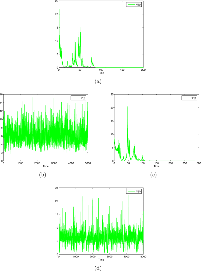
    Paths of model (3) with \(\varTheta =\{1,2\}\), \(r\equiv 0.15\), \(\mu \equiv 3\), \(\lambda \equiv 25\), \(\eta _{1}^{2}(1)=0.6\), \(\eta _{1}^{2}(2)=0.2\), \(\eta _{2}^{2}\equiv 0.16\). (a) is a path of the solution of state 1, which manifests that the extinction happens in about 85 years. (b) is a path of the solution of state 2, which manifests that the species is SP. (c) is a path of the solution of model (3) with \(\sigma =(0.8,0.2)\), which manifests that the extinction happens in about 105 years. (d) is a path of the solution of model (3) with \(\sigma =(0.2,0.8)\)

  2. (ii)

    Let \(\sigma =(0.2,0.8)\). Compute that \(\bar{\chi }=0.01>0\). Thus Theorem 2 and Theorem 3 indicate that this species in system (3) is SP and possesses a UESD (see Fig. 1(d)).

Figures 1(c) and 1(d) reflect that if the medium undulations expend much time on the extinction states such that \(\bar{\chi }+\bar{\varPi }<0\), then the dogs are in danger; if the medium undulations expend much time on the persistence states such that \(\bar{\chi }>0\), then the dogs are secure.

5 Conclusions

Evaluating the functions of environmental undulations on the evolution of species is an attractive topic in ecology [19]. The present study has taken advantage of the white noise and the Markovian switching to portray the puny undulations and medium undulations in the environment, respectively, and has put forward a stochastic population model with Allee effects under regime switching. For this model, the criteria for extinction, persistence, and the existence of a UESD have been offered. The findings uncover that these properties of system (3) highly correlate with the environmental undulations.

  • Since

    $$\begin{aligned}& \bar{\chi }=\sum_{m\in \varTheta }\sigma _{m} \chi (m), \qquad \bar{\varPi }= \sum_{m\in \varTheta }\sigma _{m} \biggl[\frac{\mu (m)}{\lambda (m)} - \frac{2(\sqrt{1+\lambda (m)\mu (m)}-1)}{\lambda ^{2}(m)} \biggr], \\& \chi (m)=r(m)-\frac{\eta _{1}^{2}(m)}{2}, \end{aligned}$$

    then for each \(m\in \varTheta \)

    $$ \frac{\mathrm{d}(\bar{\chi }+\bar{\varPi })}{\mathrm{d}\eta _{1}^{2}(m)}=- \frac{\sigma _{m}}{2}\leq 0. $$

    Accordingly, the puny undulations on the growth rate bring a hazard of extinction. This is consistent with the prior studies (see, e.g., [19]).

  • If the Markov chain \(\theta (t)\) expends much time on the persistence states such that \(\bar{\chi }>0\), then model (3) is persistent and possesses a UESD; if \(\theta (t)\) expends much time on the extinction states such that \(\bar{\chi }+\bar{\varPi }<0\), then the species represented by system (3) is dangerous.

At the end of this paper, we would like to mention that we have not examined the case \(\bar{\chi }+\bar{\varPi }>0>\bar{\chi }\). In this case, the results are too complicated to research at the present stage. This issue deserves a fuller treatment in subsequent analyses.

References

  1. Aguirre, P., González-Olivares, E., Torres, S.: Stochastic predator–prey model with Allee effect on prey. Nonlinear Anal., Real World Appl. 14, 768–779 (2013)

    Article  MathSciNet  Google Scholar 

  2. Allee, W.: Animal Aggregations: A Study in General Sociology. University of Chicago Press, Chicago (1931)

    Book  Google Scholar 

  3. Arctic Climate Impact Assessment: Impacts of a Warming Arctic—Arctic Climate Impact Assessment. Cambridge University Press, Cambridge (2004)

    Google Scholar 

  4. Bach, L., Pedersen, R., Hayward, M., Stagegaard, J., Loeschcke, V., Pertoldi, C.: Assessing re-introductions of the African Wild dog (Lycaon pictus) in the Limpopo Valley Conservancy, South Africa, using the stochastic simulation program VORTEX. J. Nat. Conserv. 18, 237–246 (2010)

    Article  Google Scholar 

  5. Boukal, D., Berec, L.: Single-species models of the Allee effect: extinction boundaries, sex ratios and mate encounters. J. Theor. Biol. 218, 375–394 (2002)

    Article  MathSciNet  Google Scholar 

  6. Clutton-Brock, T., Gaynor, D., McIlrath, G., MacColl, A., et al.: Predation, group size and mortality in a cooperative mongoose, Suricata suricatta. J. Anim. Ecol. 68, 672–683 (1999)

    Article  Google Scholar 

  7. Courchamp, F., Berec, L., Gascoigne, J.: Allee Effects in Ecology and Conservation. Oxford University Press, London (2008)

    Book  Google Scholar 

  8. Cushing, J., Hudson, J.: Evolutionary dynamics and strong Allee effects. J. Biol. Dyn. 6, 941–958 (2012)

    Article  Google Scholar 

  9. Jovanović, M., Krstić, M.: The influence of time-dependent delay on behavior of stochastic population model with the Allee effect. Appl. Math. Model. 39, 733–746 (2015)

    Article  MathSciNet  Google Scholar 

  10. Jovanović, M., Krstić, M.: Extinction in stochastic predator–prey population model with Allee effect on prey. Discrete Contin. Dyn. Syst., Ser. B 22, 2651–2667 (2017)

    MathSciNet  MATH  Google Scholar 

  11. Kang, Y.: Dynamics of a generalized Ricker–Beverton–Holt competition model subject to Allee effects. J. Differ. Equ. Appl. 22, 687–723 (2016)

    Article  MathSciNet  Google Scholar 

  12. Li, X., Jiang, D., Mao, X.: Population dynamical behavior of Lotka–Volterra system under regime switching. J. Comput. Appl. Math. 232, 427–448 (2009)

    Article  MathSciNet  Google Scholar 

  13. Li, D., Liu, M.: Invariant measure of a stochastic food-limited population model with regime switching. Math. Comput. Simul. 178, 16–26 (2020)

    Article  Google Scholar 

  14. Liebhold, A., Bascompte, J.: The Allee effect, stochastic dynamics and the eradication of alien species. Ecol. Lett. 6, 133–140 (2003)

    Article  Google Scholar 

  15. Liu, M., Bai, C.: Optimal harvesting of a stochastic mutualism model with regime-switching. Appl. Math. Comput. 375, 125040 (2020)

    Article  MathSciNet  Google Scholar 

  16. Liu, M., Deng, M.: Analysis of a stochastic hybrid population model with Allee effect. Appl. Math. Comput. 364, 124582 (2020)

    MathSciNet  MATH  Google Scholar 

  17. Liu, C., Li, H., Cheung, L.: Weak persistence of a stochastic delayed competition system with telephone noise and Allee effect. Appl. Math. Lett. 103, 106186 (2020)

    Article  MathSciNet  Google Scholar 

  18. Mao, X., Yuan, C.: Stochastic Differential Equations with Markovian Switching. Imperial College Press, London (2006)

    Book  Google Scholar 

  19. Panik, M.: Stochastic Differential Equations: An Introduction with Applications in Population Dynamics Modeling. Wiley, New York (2017)

    Book  Google Scholar 

  20. Rinella, D., Wipfli, M., Stricker, C., et al.: Pacific salmon (Oncorhynchus spp.) runs and consumer fitness: growth and energy storage in stream-dwelling salmonids increase with salmon spawner density. Can. J. Fish. Aquat. Sci. 69, 73–84 (2012)

    Article  Google Scholar 

  21. Takeuchi, Y.: Global Dynamical Properties of Lotka–Volterra Systems. World Scientific, Singapore (1996)

    Book  Google Scholar 

  22. Tobin, P., Berec, L., Liebhold, A.: Exploiting Allee effects for managing biological invasions. Ecol. Lett. 14, 615–624 (2011)

    Article  Google Scholar 

  23. Wang, K.: Stochastic Mathematical Biology Models. Science Press, Beijing (2010)

    Google Scholar 

  24. Yin, G., Zhu, C.: Hybrid Switching Diffusions: Properties and Applications. Springer, New York (2010)

    Book  Google Scholar 

Download references

Acknowledgements

We are very grateful to the referees for their careful reading and very valuable comments, which led to an improvement of our paper.

Availability of data and materials

Data sharing not applicable to this article as no datasets were generated or analysed during the current study.

Funding

ML thanks the National Natural Science Foundation of P.R. China (No. 11771174) and the Natural Science Foundation of Jiangsu Province (No. BK20170067), and “Qinglan Project” of Jiangsu Province, P.R. China.

Author information

Authors and Affiliations

Authors

Contributions

WMJ mainly finished the writing of the whole content of the paper. ML mainly finished the establishment of the model. All authors read and approved the final manuscript.

Corresponding author

Correspondence to Weiming Ji.

Ethics declarations

Competing interests

The authors declare that they have no competing interests.

Rights and permissions

Open Access This article is licensed under a Creative Commons Attribution 4.0 International License, which permits use, sharing, adaptation, distribution and reproduction in any medium or format, as long as you give appropriate credit to the original author(s) and the source, provide a link to the Creative Commons licence, and indicate if changes were made. The images or other third party material in this article are included in the article’s Creative Commons licence, unless indicated otherwise in a credit line to the material. If material is not included in the article’s Creative Commons licence and your intended use is not permitted by statutory regulation or exceeds the permitted use, you will need to obtain permission directly from the copyright holder. To view a copy of this licence, visit http://creativecommons.org/licenses/by/4.0/.

Reprints and permissions

About this article

Check for updates. Verify currency and authenticity via CrossMark

Cite this article

Ji, W., Liu, M. Dynamics of a stochastic population model with Allee effects under regime switching. Adv Differ Equ 2020, 295 (2020). https://doi.org/10.1186/s13662-020-02759-x

Download citation

  • Received:

  • Accepted:

  • Published:

  • DOI: https://doi.org/10.1186/s13662-020-02759-x

MSC

Keywords